8 Exchange Rate Systems: Fixed and Flexible

We saw in Chapter 5 that our theory of international macroeconomics has three equations representing equilibrium in the markets for goods, money, and foreign exchange. We saw in Chapter 6 that for such a theory to be useful, exactly three of the many variables in our three equations must be endogenous, and the rest exogenous. And we saw in Chapter 7 that the classification of our variables into endogenous and exogenous groups depends on (a) whether we are doing long-run analysis or short-run analysis and (b) whether we are considering a country with flexible or fixed exchange rates. This chapter focuses on exchange rate systems and the way international macroeconomic theory adapts to the exchange rate system being considered.

8.1 When Is a Country Said to Have a Fixed Exchange Rate System?

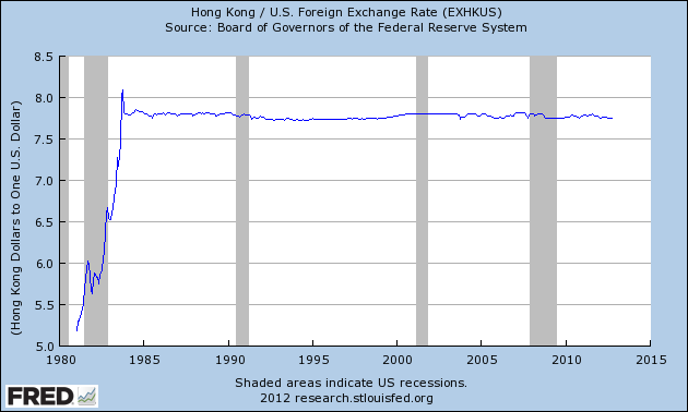
A country is said to have a fixed exchange rate system if its central bank (such as the Federal Reserve in the US or the Bank of Japan in, you guessed it, Japan) chooses a value for the nominal exchange rate ($E$) and announces that it is ready and willing to buy and/or sell any amount of the domestic currency at the rate of $E$ units of the domestic currency for one unit of the foreign currency. This action effectively fixes $E$ at the central bank’s chosen value.

Figure 8.1: Here’s an example of a fixed exchange rate. Notice that the Hong Kong dollar is fixed at about 7.80 Hong Kong dollars per U.S. dollar. Source: https://fred.stlouisfed.org/series/EXHKUS, downloaded on November 25, 2012.

To see how this works, let us talk not about currencies but about something completely different: let us talk about wheat! Assume that Bill Gates announces that he is willing to buy and/or sell any amount of wheat for $15 a bushel.¹ It is then straightforward to show that the market price will quickly become $15 per bushel. To see why, suppose the price was $18 per bushel before Bill’s announcement. As soon as Bill makes his announcement, wheat buyers, who quite understandably prefer the $15 price to the $18 price, would rush to buy Bill’s wheat at $15 per bushel and, as a result, all other wheat sellers would soon be forced to sell at Bill’s price. If, on the other hand, the price was $12 before Bill’s announcement, all sellers would sell their wheat to Bill unless other buyers start paying $15 as well. In short, the price of wheat will become whatever Bill wants it to be.

In the same way, the central bank of a nation can fix the nominal exchange rate of the domestic currency if it starts buying and selling the currency at some chosen price.

8.1.1 Money Supply Under Fixed Exchange Rates

Here, the important point to note is that under a fixed exchange rate system the central bank loses all control over $M$, the country’s money supply. To see why, suppose the US Federal Reserve announces that it will buy and/or sell dollars at 1.50 euros per dollar. If people rush to buy dollars from the Fed at that price, the Fed will have to print a fresh batch of dollars and pretty soon all those newly printed dollar bills will end up in the wallets of those who traded in their euros. That is, the US money supply ($M$), which, you may recall from Section 5.8.1, is the currency held by the public plus the value of their checking accounts, will increase. Similarly, if people choose to sell their dollars to the Fed in exchange for British pounds, the US money supply ($M$) will decrease because the dollars sold to the Fed are longer in peoples’ wallets. In short, the money supply will be whatever the people want it to be and not necessarily what the Federal Reserve wants it to be.

In other words, $M$, the money supply, becomes an endogenous variable. That is, $M$ will become a variable whose up and down movements our theory will have to explain. Just as $Y$, $C$, $EX$, $IM$, etc. are variables whose movements our theory will have to predict, $M$ will also be a variable whose movements our theory will have to predict.

To sum up, for the analysis of a fixed exchange rate system $E$ will be regarded as exogenous and constant—that is, $E_f=E$, which implies that $E_g$ is not just exogenous, it is zero—and $M$ will be regarded as endogenous.²

Figure 8.2: Here’s an example of a fixed exchange rate system that turned into a flexible exchange rate system. For about a decade until July 2, 1997, the Thai baht was pegged at about 25 to the dollar. But a currency crisis developed in 1997 and it became impossible for the central bank of Thailand to continue to keep its obligation to pay one U.S. dollar to whoever offered 25 baht in payment. At that point the baht became a flexible (or, floating) currency. It rapidly lost value—note the sharp spike in the chart—reaching the low-point of 53 baht per dollar in January 1998. Although the baht has gradually regained some of its lost value it has still not reached its pre-crisis value of 25 baht per U.S. dollar. There will be more on currency crises in a later chapter. Source: https://fred.stlouisfed.org/series/EXTHUS, downloaded on November 25, 2012.

8.2 When Is a Country Said to Have a Flexible Exchange Rate System?

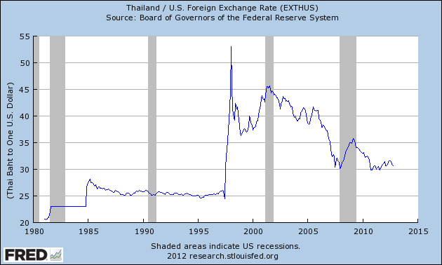
A country is said to have a flexible exchange rate system if the exchange rate ($E$) is determined in the foreign exchange market without any significant intervention or manipulation by its central bank.³ And since, in this case, the central bank does not make any promises to buy and/or sell the domestic currency at some fixed price, it can control the amount of the domestic currency that is circulating in private hands. Money supply, $M$, therefore, becomes whatever the central bank wants it to be. In other words, $M$ becomes an exogenous variable.

To sum up, the analysis of flexible exchange rate systems regards $E$ as endogenous and $M$ as exogenous.⁴

Figure 8.3: The Danish Kroner appears to float freely with respect to the U.S. dollar. But Denmark actually has a fixed exchange rate system, with its exchange rate set at about 7.45 Kroner per Euro. Source: https://www.nationalbanken.dk/en, downloaded on July 6, 2008.

Let’s assume that Bill has a large stock of wheat and a large amount of money so as to be able to deliver on his promise.↩︎
Since $M$ is endogenous, so is $M_g$, the growth rate of $M$. $M_g$ will play a role in Chapter 10, which is about long-run analysis.↩︎
For more on $E$, see Section 4.1.↩︎
$M_g$, the growth rate of $M$, will, therefore, also be exogenous. As was mentioned earlier, $M_g$ will play a role in Chapter 10, which is about long-run analysis.↩︎