13 Short-Run Predictions: Expectations and Flexible Exchange Rates
This chapter continues the analysis of the short-run macroeconomic behavior of an economy that has flexible exchange rates. The questions that concern us in this chapter share this basic format: If there is a permanent increase in [insert the name of any exogenous variable], what will happen in the short run to [insert the name of any endogenous variable]?
Recall that the consequences of temporary shocks and temporary policy changes were discussed in the previous chapter. The reason why it makes sense to analyse temporary and permanent changes in exogenous variables separately was discussed in the last paragraph of Section 11.1.3 and at the beginning of Chapter 12. The crucial difference is that permanent changes affect the future—and therefore our expectation of what our future will be—whereas temporary changes don’t.
13.1 Fiscal Policy
Let us jump right in and try to analyze the short-run effects of a permanent increase in government spending.
13.1.1 The Primary Effect
We begin by recalling—from Section 12.4.1 or the \(G\)-row of table Table 12.1 —the short-run effects of a temporary increase in government spending. The \(DD\) curve, which represents all pairs of values of real output (\(Y\)) and the exchange rate (\(E\)) that keep the goods market in equilibrium, shifts to the right. The \(AA\) curve, which represents all pairs of values of real output (\(Y\)) and the exchange rate (\(E\)) that keep the money and foreign currency markets in equilibrium, stays put. As a result, there are increases in output, consumption, and the interest rate (\(Y\uparrow\), \(C\uparrow\), \(R\uparrow\)), and decreases in net exports, the nominal exchange rate, and the real exchange rate (\(NX\downarrow\), \(E\downarrow\), \(q\downarrow\)).
Needless to say, these effects are temporary. A temporary increase in government spending will, by definition, soon be reversed. Therefore, \(G\) will return to its original level. The \(DD\) curve will return to its original position, and all endogenous variables will return to their original values.
On the other hand, when the increase in government spending is permanent, the \(DD\) curve will shift permanently to the right. Therefore, the temporary changes in \(Y\), \(C\), \(R\), \(NX\), \(E\), and \(q\) that we saw two paragraphs back will now be permanent.
I will call these effects of a permanent increase in government spending the primary effect. The primary effect of a permanent increase in government spending is the same as the short-run effect of a temporary increase in government spending that we saw in the \(G\)-row of table Table 12.1.
In general, the primary short-run effect of a permanent increase in any given exogenous variable \(X\) on any endogenous variable \(Z\) is identical to the short-run effect of a temporary increase in \(X\) on \(Z\), and this effect can be seen in the \(X\)-row and \(Z\)-column of Table 12.1.
13.1.2 The Secondary Effect
So far, it looks as if distinguishing between permanent and temporary changes in an exogenous variable is a waste of time. It looks as if a permanent increase in \(G\) has the same effects as a temporary increase in \(G\), except that the effects of former are permanent and the effects of the latter are temporary.
But actually there’s more to the story. A permanent increase in \(G\) will reduce the long-run equilibrium value of \(E_f\), which will lead to an immediate decrease in \(E_f^e\), which will have additional short-run effects of its own (on our endogenous variables).
Feeling dizzy? Let’s go over this step by step.
The \(G\)-rows of tables Table 9.1 and Table 10.1 summarize the long-run effects of a permanent increase in government spending. Note in particular that the long-run equilibrium value of the future value of the foreign currency decreases (\(E_f\downarrow\)). Now recall from Section 7.3 that in short-run analysis it is assumed that the expected value of \(E_f\) is equal to its long-run equilibrium value: that is, \(E_f^e=E_{fLR}\). Therefore, it follows that, as soon as the permanent increase in government spending occurs, people will realize that \(E_f\) will eventually fall, and, consequently, they will revise downward their expectation of the future value of the foreign currency (\(E_f^e\downarrow\)).
Will this decrease in \(E_f^e\) have further effects on our endogenous variables? Indeed, it will. Recall from Section 12.4.3 and the \(E_f^e\)-row of table Table 12.1 that a temporary decrease in \(E_f^e\) will temporarily affect various endogenous variables: \(Y\downarrow\), \(C\downarrow\), \(R\downarrow\), \(NX\downarrow\), \(E\downarrow\), and \(q\downarrow\). Therefore, a permanent decrease in \(E_f^e\) will have the same effects, only this time the effects will be permanent.
I will call these effects of a permanent increase in government spending the secondary effect, because it works indirectly by influencing people’s expectations (\(E_f^e\)).
In general, the indirect short-run effect of a permanent increase in any given exogenous variable \(X\) on any endogenous variable \(Z\) can be deduced as follows: First, look at the \(X\)-row and \(E_f\)-column of Table 10.1 to see whether the long-run equilibrium value of \(E_f\) will increase or decrease if \(X\) increases.1 Second, look at the \(E_f^e\)-row of table Table 12.1 to see whether the endogenous variable \(Z\) will increase or decrease. In this way, we can deduce the secondary effect of \(X\) on \(Z\).
Actually, the process of figuring out the secondary effect of exogenous variable \(X\) on endogenous variable \(Z\) can be further simplified. The second step in the last paragraph is actually unnecessary. To see why, note that the \(E_f^e\)-row of table Table 12.1 has all plus (\(+\)) signs, indicating that any change in \(E_f^e\) causes all the relevant endogenous variables to change in the same direction. Therefore, if you know that an increase in \(X\) leads to an increase (respectively, a decrease) in \(E_f^e\), you can immediately conclude that the secondary effect of an increase in \(X\) will lead to an increase (respectively, a decrease) in all endogenous variables including \(Z\).
13.1.3 The Total Effect
It is now time to add the primary and secondary effects of a permanent increase in government spending and thereby deduce the total effects.
- primary effect of a permanent increase in \(G\) (same as the temporary effects in table Table 12.1): \(Y\uparrow\), \(C\uparrow\), \(R\uparrow\), \(NX\downarrow\), \(E\downarrow\), \(q\downarrow\)
- effect of a permanent increase in \(G\) on expectations (see Table 10.1): \(E_f^e\downarrow\)
- secondary effect of a permanent increase in \(G\) (same as the effect on \(E_f^e\)): \(Y\downarrow\), \(C\downarrow\), \(R\downarrow\), \(NX\downarrow\), \(E\downarrow\), \(q\downarrow\)
- total effect: \(Y?\), \(C?\), \(R?\), \(NX\downarrow\), \(E\downarrow\), \(q\downarrow\), where “\(?\)” stands for an ambiguous effect
Note that when the direct and indirect effects go in opposite directions, the total effect is, unfortunately, ambiguous.
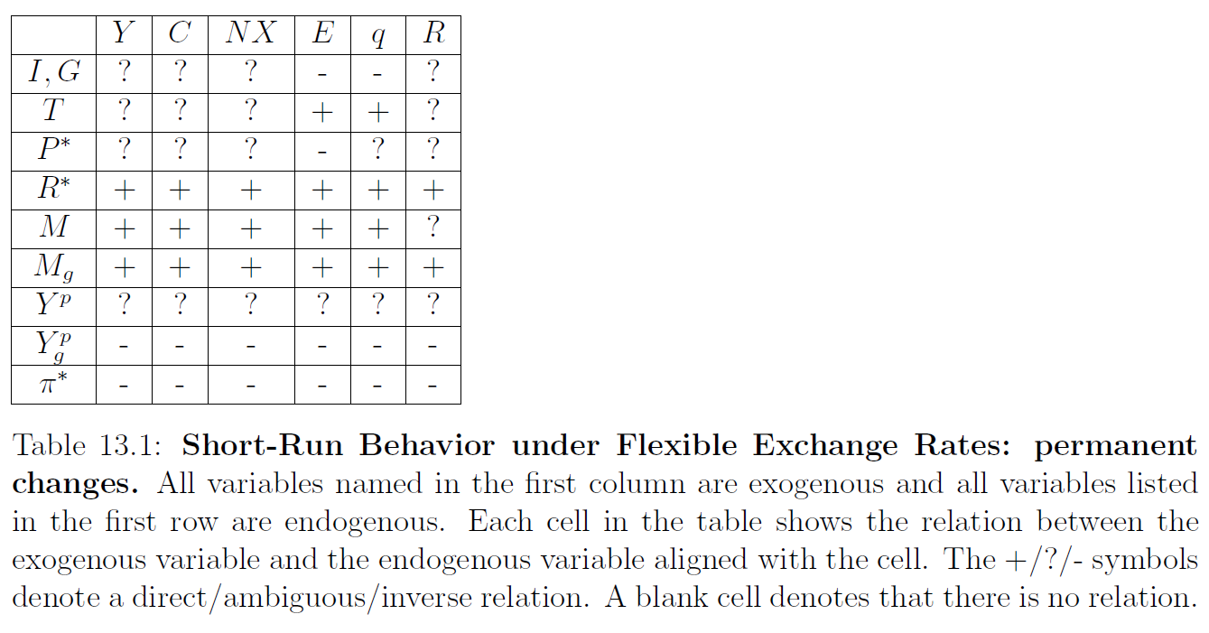
The total effects are summarized in the \(G\)-row of table Table 13.1. It is straightforward to check that the short-run effects of a permanent increase in business investment (\(I\uparrow\)) are identical, which is why \(G\) and \(I\) share the same row in table Table 13.1.
Note that the primary and secondary effects of a permanent increase in government spending on real output run in opposite directions. The primary effect leads to higher \(Y\) and the secondary effect leads to lower \(Y\). As a result, the effect of a permanent fiscal stimulus on output is weaker than that of a temporary stimulus. Indeed, I cannot rule out the possibility that the secondary effect may be stronger than the primary effect, in which case a fiscal stimulus can be counterproductive and lead to lower real output.
13.2 More Examples
In general, the short-run effect of a permanent increase in any given exogenous variable \(X\) on any given endogenous variable \(Z\) can be deduced as follows:
- The primary short-run effect of a permanent increase in \(X\) is shown in the \(X\)-row and \(Z\)-column of table Table 12.1. Make a note of this effect.
- The effect of a permanent increase in \(X\) on \(E_f^e\) is shown in the \(X\)-row and \(E_f\)-column of Table 10.1. Make a note of this effect.
- The secondary short-run effect of a permanent increase in \(X\) on \(Z\) is the same as \(X\)’s effect on \(E_f^e\) that we saw in the previous step.
- The total short-run effect is the sum of the primary and secondary effects. If these two effects are pulling in opposite directions, the total effect is “ambiguous” or “\(?\)”.
To illustrate, let us consider a permanent increase in money supply (\(M\)).
- The primary short-run effects of a permanent increase in \(M\) are shown in the \(M\)-row of table Table 12.1: \(Y\uparrow\), \(C\uparrow\), \(R\uparrow\), \(NX\uparrow\), \(E\uparrow\), \(q\uparrow\)
- The effect of a permanent increase in \(M\) on \(E_f^e\) is shown in the \(M\)-row and \(E_f\)-column of Table 10.1: \(E_f^e\uparrow\)
- The secondary short-run effects of a permanent increase in \(M\) are the same as \(M\)’s effect on \(E_f^e\): \(Y\uparrow\), \(C\uparrow\), \(R\uparrow\), \(NX\uparrow\), \(E\uparrow\), \(q\uparrow\)
- The total short-run effect is the sum of the primary and secondary effects: \(Y\uparrow\), \(C\uparrow\), \(R\uparrow\), \(NX\uparrow\), \(E\uparrow\), \(q\uparrow\)
This is shown in the \(M\)-row of table Table 13.1.
Note that the primary effect of monetary policy is reinforced or strengthened by the secondary effect. This implies that the short-run impact of a monetary stimulus will be stronger if it is permanent rather than temporary.
For another example, let us consider the short-run effect of a permanent increase in the foreign inflation rate (\(\pi^*\uparrow\)).
- There are no primary short-run effects of a permanent increase in \(\pi^*\), as table Table 12.1 does not even have a \(\pi^*\)-row!
- The effect of a permanent increase in \(\pi^*\) on \(E_f^e\) is shown in the \(\pi^*\)-row and \(E_f\)-column of Table 10.1: \(E_f^e\downarrow\)
- The secondary short-run effects of a permanent increase in \(\pi^*\) are the same as \(\pi^*\)’s effect on \(E_f^e\): \(Y\downarrow\), \(C\downarrow\), \(R\downarrow\), \(NX\downarrow\), \(E\downarrow\), \(q\downarrow\)
- The total short-run effect is the sum of the primary and secondary effects: \(Y\downarrow\), \(C\downarrow\), \(R\downarrow\), \(NX\downarrow\), \(E\downarrow\), \(q\downarrow\)
This is shown in the \(\pi^*\)-row of table Table 13.1. Note that, as there is no primary short-run effect of an increase in the foreign inflation rate, its total short-run effect consists of the secondary effect of \(\pi^*\) on \(E_f\) and, therefore, on \(E_f^e\). This is also true for the rows in table Table 13.1 for \(Y^p\), \(M_g\), and \(Y^p_g\). In the case of \(Y^p\) there is an additional complication. A quick look at Table 10.1 will show that the long-run effect of an increase in potential output on the future value of the foreign currency is ambiguous. Therefore, the effect of \(Y^p\) on \(E_f^e\) is ambiguous. And, therefore, the indirect effects of \(Y^p\) on our endogenous variables are ambiguous as well.
Using the step-by-step process illustrated in the three examples above for the \(G\), \(M\), and \(\pi^*\) rows of table Table 13.1, the contents of all the other cells can be verified. I leave that task to the reader.
13.3 Conclusion
From the point of view of policy making, it is important to note that the short-run effect of a permanent change in government spending and/or taxes is weaker than—or, possibly, even the reverse of—a temporary change. A temporary increase in government spending on, say, the construction of roads, bridges, etc., or a temporary tax cut stimulates demand and leads to an increase in output and the creation of new jobs for the jobless. But there is less reason to be optimistic about the short-run stimulative effect of a permanent increase in government spending or a permanent tax cut. A permanent fiscal stimulus will, in the long run, raise the value of the domestic currency (\(E_f\downarrow\)). Knowing this, people will revise upward their expectations about the future value of the domestic currency (\(E_f^e\downarrow\)), and will do so immediately. This will reduce the competitiveness of domestic goods—as can be checked from the \(E_f^e\)-row of table Table 12.1, \(q\downarrow\), which implies that foreign goods become relatively cheaper—and lead to a fall in net exports, lower output, and fewer jobs.
In other words, a permanent fiscal stimulus creates jobs and destroys jobs at the same time, and the overall effect could go either way.
Of course, a lot depends on the assumption that expectations (\(E_f^e\)) are tightly linked to the long-run equilibrium outcome (\(E_{fLR}\)). I have assumed that as soon as a permanent increase in government spending is announced, the people will figure out that \(E_f\) will end up higher than they had previously thought. As a result, \(E_f^e\) will increase rightaway. This is at the root of the adverse secondary effect that says that net exports will fall and, consequently, output will shrink. But if, in the real world, people do not put two and two together and do not revise their expectations immediately after the increase in \(G\), then the adverse secondary effect would not happen, and the fiscal stimulus will work unobstructed.
A monetary stimulus, in stark contrast, has a stronger effect when it is permanent. Perhaps a policy lesson that we can take from this chapter is that a government facing a recession should use a temporary fiscal stimulus and a permanent monetary stimulus.
Actually, \(E_f^e\) may stay unchanged. It may even be that the effect of \(X\) on \(E_f\) is ambiguous. I am just trying to keep the discussion simple.↩︎