7  The Long Run and the Short Run

7.1 In Our Three Basic Equations, Which Variables Are Exogenous and Which Are Endogenous?

My discussion of international macroeconomic theory has, so far, described three equations that represent equilibrium in the goods, money, and foreign exchange markets.¹ So, for the theory to work, there would have to be exactly three endogenous variables.² So, we need to start figuring out which variables in those three equations are exogenous and which are endogenous and check how many endogenous ones there are.

The list of variables that you have seen so far is already pretty long: \(G\), \(T\), \(M\), \(q\), \(Y\), \(C\), \(I\), \(NX\), \(EX\), \(IM\), \(E\), \(E^e_f\), \(R\), \(R^*\), \(P\), and \(P^*\). The question is: Which of these are endogenous and which are exogenous?³

The variables that will always be exogenous in these lectures are \(I\), \(G\), and \(T\). Moreover, all variables that describe the foreign country (\(R^*\) and \(P^*\)) will also be regarded as exogenous.

The variables that will always be endogenous in these lectures are \(Y\), \(C\), \(I\), \(NX\), \(EX\), \(IM\), \(q\), and \(R\).

As for the other variables, whether they are exogenous or endogenous will depend on two issues:

• Do we want to do long-run analysis or short-run analysis? and
• Does the domestic economy have a fixed exchange rate system or a flexible exchange rate system?

In this chapter, I will discuss the distinction between long-run and short-run analysis. The next chapter looks at the distinction between flexible and fixed exchange rate systems.

7.2 What Is Long-Run Analysis?

In the long-run analysis of equilibrium in the markets for goods, foreign exchange, and money, the following simplifying assumptions are made:

• Full Employment : all productive resources of the economy are assumed to be fully employed in the long run. That is, an economy’s real GDP (\(Y\)) is assumed to be equal to its potential real GDP (\(Y^p\)).⁴
• Perfect Foresight : people’s expectations are assumed to be accurate. Specifically, it is assumed that the actual future value of the foreign country’s currency (\(E_f\)) will be equal to the expected future value of the foreign country’s currency (\(E^e_f\)). Equivalently, it is assumed that the actual rate of growth of the value of the foreign country’s currency (\(E_g\equiv(E_f-E)/E\)) is equal to the expected rate of growth of the value of the foreign country’s currency (\(E^e_g\equiv(E^e_f-E)/E\)).⁵

Perfect foresight is a simpler form of a common assumption in economics called rational expectations . Economists are aware of the fallibility of their forecasts.⁶ Nevertheless, it makes sense to assume that although expectations about the future value of a variable will at times exceed the actual outcome and at times be less than the actual outcome, they will on average be reasonably accurate. There is no a priori reason to believe that we will consistently overestimate (or, consistently underestimate) what the exchange value of the dollar will be in the future.

7.2.1 Potential Real Gross Domestic Product

Figure 7.1: Potential Output The red graph represents the U.S. Congressional Budget Office’s estimates of potential real GDP (in billions of chained 2000 dollars). The blue graph represents actual real GDP. The excess of potential GDP over actual GDP is referred to as the GDP gap. The gray bars in the figure represent the periods of recession in the U.S. economy. Actual GDP is typically less than potential GDP during recessions. Source: Data on real GDP was downloaded from https://fred.stlouisfed.org/series/GDPC1 and data on potential real GDP was downloaded from https://fred.stlouisfed.org/series/GDPPOT, both on November 25, 2012.

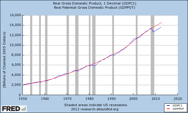
As was just mentioned, a country’s real GDP is assumed to be equal to its real potential GDP in the long run. Potential Real GDP is the real GDP that would be produced if the utilization of the resources of the economy were at normal levels. Actual real GDP, \(Y\), is less than potential real GDP when resources are under-utilized, as in a recession. On the other hand, if resource utilization is at abnormally high levels, as in a booming economy, actual real GDP could exceed potential real GDP.

An economy’s potential GDP depends on several factors. Potential GDP will be high if (a) the quantity and quality of the productive resources that the country is endowed with are high, (b) it can purchase from other countries at a low price the resources it does not have, (c) it has access to advanced technology, and (d) it has the economic policies and cultural institutions that encourage the efficient utilization of all resources. However, for the purposes of this book, \(Y^p\) will be regarded as exogenous, something as inscrutable as the weather.

The Congressional Budget Office, an arm of the United States Congress, publishes estimates of America’s potential real GDP.⁷ Potential GDP is a conceptual notion that cannot be directly observed. But that does not mean that it cannot be reliably estimated. See figure Figure 7.1 for a look at the CBO’s estimates of America’s potential real GDP.

7.3 What Is Short-Run Analysis?

In short-run analysis I make the following simplifying assumptions:

• Fixed Prices : The variables \(P\), \(P^*\) are assumed to be exogenous and constant.
• Long-Run Expectations : People’s expectations about the future value of a variable (that is, variables such as \(E^e_f\) and \(E^e_g\)) are assumed to be equal to its long-run value. For example, if \(E_{fLR}\) represents the value of the foreign country’s currency in long-run equilibrium, then \(E^e_f=E_{fLR}\) is assumed true in the short run.

The assumptions about expectations formation for the long and short runs can, therefore, be combined into one simple statement: \(E^e_f=E_{fLR}\) irrespective of whether we are doing long-run analysis or short-run analysis.

Shackleton, Robert. 2018. Estimating and Projecting Potential Output Using CBO’s Forecasting Growth Model. Congressional Budget Office.

---

1. See Section 5.10.

2. See Theorem 6.1 in Section 6.1.3.

3. Recall from Section 6.1.1 and Section 6.1.2 that endogenous variables are the variables whose ups and downs are explained by the theory and exogenous variables are the variables that the theory does not consider to be any of its business.

4. I realize that I haven’t discussed potential real GDP so far, but I will do so shortly. But the key point here is that potential real income will be assumed exogenous throughout this book. So, the \(Y=Y^p\) assumption of long-run analysis can be used to replace the endogenous variable \(Y\) by the exogenous variable \(Y^p\). As you will see in Chapter 9, this replacement of an endogenous variable by an exogenous variable will greatly simplify the analysis.

5. Recall from Section 2.3.1 that the current value of any variable \(x\) is also denoted \(x\), the future value of \(x\) is denoted \(x_f\), and the growth rate of \(x\) is denoted \(x_g=(x_f-x)/x\). The expected appreciation of the foreign country’s currency was defined in Equation 5.11 of Section 5.9.2.

6. Partly because non-economists won’t stop reminding them.

7. For details, see CBO’s Method for Estimating Potential Output: An Update, Congressional Budget Office, August 2001, https://www.cbo.gov/sites/default/files/107th-congress-2001-2002/reports/potentialoutput.pdf and Shackleton (2018) (online).