10 Long-Run Predictions: The Nominal World

This chapter continues the discussion of long-run equilibrium that I began in the last chapter. That chapter had focused on real variables , which are variables that would be meaningful even in a discussion of a barter-based world in which nobody uses cash as well as a world in which people use cash. This chapter focuses on nominal variables , such as the nominal exchange rate and the rate of inflation, which mean something only in an economy in which people use money.

10.1 The Classical Dichotomy and Monetary Neutrality

The notion that it is theoretically useful to classify economic variables into real and nominal variables is called the classical dichotomy . The related idea that real and nominal variables can be discussed separately because changes in $M$, the quantity of money, do not affect real variables, is called monetary neutrality .¹

The neutrality of money in the long run made it possible for me to limit Chapter 9 to a discussion of only the real variables. We will see in this chapter, however, that although real variables can be discussed without mentioning nominal variables, the reverse is not true: changes in real exogenous variables can affect nominal endogenous variables.

Classical economists were aware—as are today’s economists—that monetary neutrality made sense in the long run but not in the short run. As later chapters will show, any discussion of short-run international macroeconomics must juggle real and nominal variables simultaneously.

10.2 Some Math Results on Growth Rates

Before we can tackle the long-run behavior of nominal endogenous variables, we need to do some math.

Recall from Section 2.3.1 that the growth rate of a variable is denoted here by the symbol for that variable with the letter $g$ attached as a subscript. It can then be shown that:

Theorem 10.1 (Growth rate of a product of variables) If $z=x\cdot y$, then $z_g=x_g+y_g$. That is, the growth rate of the product of a bunch of variables is equal to the sum of the growth rates of those variables.

Suppose the number of families in your town increases from 100 to 110, a 10% increase. Suppose the average number of people per family increases from 5 to 6, a 20% increase. Therefore, the population of your town, which is given by the product of the number of families and the average family size, increases from 500 to 660, a 32% increase. Note that 32 is approximately equal to $20+10=30$, the answer you’d get if you followed Theorem 10.1.

Suppose instead that the number of families decreases from 100 to 90, a 10% decrease or, equivalently, a $-10$% increase. In this case, the total population increases from 500 to 540, an 8% increase. Again, note that 8 is approximately equal to $20+(-10)=10$, the answer according to Theorem 10.1.²

A related result can also be proved:

Theorem 10.2 (Growth rate of a ratio of variables) If $z=x/y$, then $z_g=x_g-y_g$. That is, the growth rate of the ratio of a pair of variables is equal to the growth rate of the variable in the numerator minus the growth rate of the variable in the denominator.

10.3 Changes in the Real Exchange Rate

Recall from Equation 4.1 that the real exchange rate is $q=E\cdot P^*/P$. Theorem 10.1 above implies that the growth rate of $E\cdot P^*$ is $(E\cdot P^*)_g=E_g+P_g^*=E_g+\pi^*$, where $\pi^*\equiv P^*_g$ is the foreign inflation rate. Theorem 10.2 then implies that the growth rate of $q=E\cdot P^*/P$ is $q_g=(E\cdot P^*)_g-P_g=(E\cdot P^*)_g-\pi$, where $\pi\equiv P_g$ is the domestic inflation rate. It then follows that \[ q_g=E_g+\pi^*-\pi. \tag{10.1}\]

Figure 10.1: Relative Purchasing Power Parity assumes that $q$ is constant ($q_g=0$) but allows instantaneous changes in $q$ at isolated points in time.

10.4 Purchasing Power Parity, Absolute and Relative

Recall the discussion of the law of one price—also called absolute purchasing power parity—in Section 5.6.4. Absolute purchasing power parity says that $q=1$—see Equation 5.7. That is, not only must the real exchange rate be constant, it must be equal to one. The argument behind absolute purchasing power parity—which was discussed in Section 5.6.3 —is typically regarded as theoretically interesting and even cogent, but factually shaky. On the other hand, relative purchasing power parity, a less stringent version of the same idea, is widely accepted. Relative purchasing power parity is the assumption that in the long run the real exchange rate ($q$) is constant over time, though not necessarily equal to one.

For the rest of this chapter, I will assume relative purchasing power parity or, equivalently,³ \[ q_g=0. \tag{10.2}\]

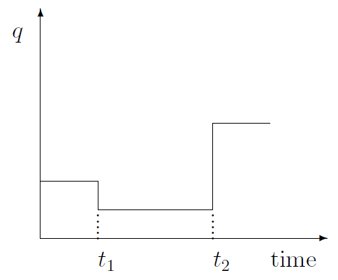
Now, this may sound like a contradiction, but please hear me out. The assumption that $q$ is constant over time does not mean that $q$ can never change. Take a look at Figure 10.1. Except for two fleeting moments in time—$t_1$ and $t_2$—$q$ is indeed constant. Of course $q$ does change at $t_1$ and $t_2$. But these changes are perfectly consistent with the assumption of relative purchasing power parity.

A quick glance at the $q$-column of Table 9.1 will serve as a reminder that permanent changes in $I$, $G$, $T$, and $Y^p$ lead to long-run changes in $q$. Therefore, my assumption that $q$ is constant over time except for occasional instantaneous changes at isolated points in time, requires the additional assumption that $I$, $G$, $T$, and $Y^p$ must be constant over time, except for rare instantaneous changes.

10.4.1 Exchange Rates: it’s a race between our inflation rate and their inflation rate

Equation 10.1 and Equation 10.2 imply something very stark about the long-run behavior of the nominal exchange rate:

\[ E_g=\pi-\pi^*. \tag{10.3}\]

In other words, the percentage increase in the value of the foreign currency is equal to the excess of the domestic inflation rate over the foreign inflation rate. If US inflation is 5% and European inflation is 3%, then the price of one euro (measured in dollars) will rise by 2%. Nothing else matters. It’s that simple.

10.5 Uncovered Interest Parity in the Long Run

Recall, from Section 5.9.2.1, that for the foreign exchange market to be in equilibrium, uncovered interest rate parity, $R=R^* + E^e_g$, must be satisfied. Moreover, recall, from Section 7.2, that in long-run equilibrium expectations are assumed to be accurate. In particular, it is assumed that $E^e_g=E_g$. By inserting this result and Equation 10.3 into the uncovered interest parity equation, we get \[ R=R^* + E^e_g=R^* + E_g=R^*+\pi-\pi^*. \tag{10.4}\]

Recall from Section 7.1 that $R^*$ and $\pi^*$ are assumed to be exogenous. I will now further assume that they are constant, meaning that they stay unchanged at their historical levels as the years pass by.

Consequently, one prediction from the equation above is that any change in the domestic inflation rate ($\pi$) must be accompanied by an identical change in the domestic interest rate ($R$). This idea is known as the Fisher effect, after the economist Irving Fisher (1867–1947).

Finally, I will also assume that the domestic inflation rate ($\pi$) is constant in the long-run equilibrium. Equation 10.4 then implies that the domestic nominal interest rate must be constant as well.

10.6 Money Market Equilibrium

Recall from Section 5.8 that equilibrium in the money market can be represented by Equation 5.9. The full-employment assumption of long-run analysis—i.e., $Y=Y^p$; see Section 7.2 —then implies: \[ M=L(R)\cdot P\cdot Y^p, \tag{10.5}\]

where $L(R)$, the propensity for liquidity, is inversely related to $R$, the nominal interest rate.⁴

A straightforward application of Theorem 10.1 of Section 10.2 to Equation 10.5 implies $M_g=L_g+\pi+ Y^p_g$, where $L_g$ and $Y^p_g$ are simply the growth rates of $L$ and $Y^p$. As we saw in Section 10.5 above, under my assumptions, $R$ is constant in long-run equilibrium. Therefore, $L(R)$ must be constant too, implying $L_g=0$. Therefore, we get \[ M_g=\pi+ Y^p_g. \tag{10.6}\]

10.7 The Economy’s Growth Rate

In these lectures, potential output ($Y^p$) and its growth rate ($Y^p_g$) are assumed to be exogenous. Moreover, recall from Section 10.4, that the assumption of relative purchasing power parity requires the assumption that $Y^p_g=0$.

Under absolute purchasing power parity, on the other hand, changes in $Y^p$ have no effect on $q$, which is always $q=1$ anyway. Therefore, under absolute purchasing power parity, there is no need to assume $Y^p_g=0$.

10.8 A Flexible Exchange Rate System

I will now try to describe the long-run behavior of nominal variables in an economy that has a flexible exchange rate system.

Recall from Section 8.2 that in a flexible exchange rate system the nominal value of the foreign currency, $E$, is endogenous and the quantity of money in the domestic economy, $M$, is exogenous. It follows that $E_g$, the rate of growth (or appreciation) of the price of the foreign currency, must also be endogenous, and $M_g$, the growth rate of he quantity of money, must be exogenous.

10.8.1 Inflation

Equation 10.6 can be rewritten as \[ \pi=M_g-Y^p_g. \tag{10.7}\]

Note that $M_g$ and $Y^p_g$ are both exogenous. Therefore, this equation tells us all that can be said about the long-run inflation rate: $\pi$ is directly affected by $M_g$, inversely affected by $Y^p_g$, and unaffected by all other exogenous variables.⁵ In fact, the effects are one-for-one: If the growth in the money supply speeds up by two percentage points (or if the growth of GDP slows down by two percentage points), inflation will speed up by the same two percentage points.

Inflation, in the long run, is a race between money supply and real GDP. Imagine what would happen if the monetary authorities of a country decide one day to print massive quantities of currency and drop them all across the country from helicopters. Once they have recovered from the initial shock, the people will rush to grab the money as fast as they possibly can. Cash-strapped people would rush immediately to the mall to buy stuff. Others would deposit the money in their bank accounts. But their bank managers would, as soon as possible, lend the money out to borrowers, because banks make money by lending their depositors’ money at interest rates that are higher than what the depositors are being paid. So, one way or another, the helicopter money would end up in the hands of eager shoppers. But the cruel irony is that the amount of stuff available for people to buy has not changed; after all, the amount of labor, land, and other productive resources did not magically increase when the money rained down from the helicopters. Therefore, the people will end up spending more money on the same amount of goods, which is another way of saying that all that they will do is bid up the prices of goods!

The amount of goods produced and purchased will remain unaffected by the helicopter money. And, indeed, why would it? If it were possible to increase production by simply printing money and dropping it everywhere from helicopters, every country in the world would have easily attained a princely standard of living. The fact that there are many poor people and poor countries all over the world is proof that printing currency bills cannot lead to higher output. All it does is raise prices.

Of course, $Y^p$ could increase for other reasons, such as increases in the labor force, the accumulation of capital equipment, technological progress, etc. If real potential GDP increases at the annual rate of 3.5% and the money supply increases at the rate of 5.0%, then Equation 10.7 tells us that inflation will run at the annual rate of $5.0-3.5=1.5$%.

Note that $Y^p_g$, a real variable, does have an effect on $\pi$, a nominal variable. This illustrates the point made in my discussion of monetary neutrality in Section 10.1: real variables can be discussed without mentioning any nominal variables, but the reverse is not true.

Recall from Section 10.7 above that $Y^p_g=0$ must be assumed when relative purchasing power parity is assumed. In that case the rate of inflation is the same as the rate at which the quantity of money is increasing in the domestic economy: that is, $\pi=M_g$.

Table 10.1: **Behavior of Nominal Variables Under Flexible Exchange Rates in the Long Run.** All variables named in the first column are exogenous and all variables listed in the first row are endogenous. Each cell in the table shows the relation between the exogenous variable and the endogenous variable aligned with the cell. The +/?/- symbols denote a direct/ambiguous/inverse relation. A blank cell denotes that there is no relation. The $Y^p_g$ row is meaningful only under absolute purchasing power parity.

10.8.2 Appreciation of the Nominal Exchange Rate

By using Equation 10.6, Equation 10.3 can be rewritten as \[ E_g=M_g-Y^p_g-\pi^*. \tag{10.8}\]

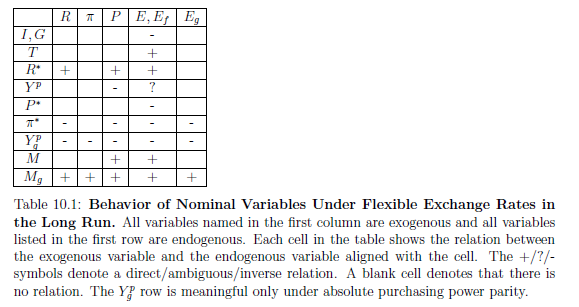
As all three variables on the right-hand side of this equation are exogenous, this equation tells us all that can be said about the rate of appreciation of the foreign currency: $E_g$ is inversely affected by $\pi^*$ and $Y^p_g$, directly affected by $M_g$, and unaffected by all other exogenous variables. These ceteris paribus effects are shown in the $E_g$-column of Table 10.1.

10.8.3 The Nominal Interest Rate

Using Equation 10.6, Equation 10.4 can be rewritten as \[ R=R^*-\pi^*- Y^p_g+M_g. \tag{10.9}\]

Again, note that all variables on the right-hand side of this equation are exogenous. It follows that $R$, the nominal interest rate, is directly affected by $R^*$ and $M_g$, inversely affected by $\pi^*$ and $Y^p_g$, and unaffected by all other exogenous variables. These ceteris paribus effects are shown in the $R$-column of Table 10.1.

10.8.4 The Price Level

Equation 10.5 and Equation 10.9 can be combined into: \[ P=\frac {M}{L(R^*-\pi^*- Y^p_g+M_g)\cdot Y^p}. \tag{10.10}\]

Note that the above equation expresses the long-run equilibrium price level entirely in terms of exogenous variables. Therefore, the above equation tells us all that can be said about the price level.

Recall from Section 5.8.4 that $L$ is inversely related to $R=R^*-\pi^*- Y^p_g+M_g$. Therefore, an increase in either $R^*$ or $M_g$ or both (or a decrease in either $\pi^*$ or $Y^p_g$ or both) will raise $R$, reduce $L$, and, therefore, raise $P$. It follows that the price level, $P$, is directly affected by $M$, $R^*$ and $M_g$, inversely affected by $Y^p$, $Y^p_g$, and $\pi^*$, and unaffected by all other exogenous variables. These ceteris paribus effects are shown in the $P$-column of Table 10.1.

10.8.5 The Nominal Exchange Rate

Equation 4.1, which defines the real exchange rate, can be rewritten as \[ E=\frac {q\cdot P}{P^*}. \tag{10.11}\]

Consider the exogenous variables $I$, $G$ and $T$. A quick look at the previous section shows that they do not affect $P$. Therefore, their effects on $E$ would be identical to their effects on $q$, which are described in Section 9.4 and shown in the $q$-column of Table 9.1. %Under absolute purchasing power parity, however, $q=1$ always, which implies $E=P/P^*$.

The foreign price level, $P^*$, affects neither $q$—see Section 9.4 —nor $P$—see Section 10.8.4. It is then obvious from Equation 10.11 that $E$ is inversely related to $P^*$.

An increase in $R^*$ or $M$ or $M_g$ or a decrease in $\pi^*$ or $Y^p_g$ (or some combination of these changes) will increase $P$, as we just saw in Section 10.8.4; have no effect on $q$, according to Section 9.4; and have no effect on $P^*$, which is exogenous anyway. Therefore, by Equation 10.11, $E$ will increase.

% Section 9.4 makes it clear that $Y^p_g$, $M$, and $M_g$ do not affect $q$. As $P^*$ is exogenous, Equation 10.11 implies that $Y^p_g$, $M$, and $M_g$ can affect $E$ only through their effects on $P$. According to Section 10.8.4, an increase in $M$ or $M_g$ or a decrease in $Y^p_g$ will lead to an increase in $P$, which, by Equation 10.11, will lead to an increase in $E$.

Finally, an increase in $Y^p$ leads to an increase in $q$ and a decrease in $P$ and leaves $P^*$, which is exogenous anyway, unchanged. Therefore, by Equation 10.11, the effect of $Y^p$ on $E$ is ambiguous.

To summarize, the nominal exchange rate, $E$, is inversely affected by $I$, $G$, $P^*$, $\pi^*$, and $Y^p_g$; directly affected by $T$, $R^*$, $M$, and $M_g$; ambiguously affected by $Y^p$; and unaffected by all other exogenous variables. These ceteris paribus effects are shown in the $E$-column of Table 10.1.

10.8.6 The Future Value of the Nominal Exchange Rate

Can we make any predictions about the future value of the nominal exchange rate ($E_f$)?

As we saw in Section 2.3.1, the rate of appreciation of the nominal exchange rate is $E_g\equiv (E_f-E)/E$, which implies $E_f=(1+E_g)\cdot E$.

Now, let us consider the long-run behavior of $E_g$ and $E$, as discussed in Section 10.8.2 and Section 10.8.5 and summarized in the $E$ and $E_g$ columns of Table 10.1. Note that there is no exogenous variable whose effect on $E_g$ contradicts its effect on $E$. Therefore, for every exogenous variable, its effect on $E$ will be the same as its effect on $E_f=(1+E_g)\cdot E$. This is why the $E$ and $E_f$ columns of Table 10.1 are the same.

To summarize, the future value of the nominal exchange rate, $E_f$, is inversely affected by $I$, $G$, $P^*$, $\pi^*$, and $Y^p_g$; directly affected by $T$, $R^*$, $M$, and $M_g$; ambiguously affected by $Y^p$; and unaffected by all other exogenous variables.

This completes my discussion of the long-run behavior of nominal variables in an economy that has a system of flexible exchange rates. The results are summarized in Table 10.1.

10.9 A Fixed Exchange Rate System

I will now try to describe the long-run behavior of the nominal variables in an economy that has a system of fixed exchange rates.

Recall from Section 8.1 that in a fixed exchange rate system the nominal value of the domestic currency, $E$ is exogenous (because, after all, it is fixed!) and the quantity of money, $M$, is endogenous. It follows that $M_g$, the growth rate of he quantity of money, is endogenous as well.

Table 10.2: **Behavior of Nominal Variables Under Fixed Exchange Rates in the Long Run.** All variables named in the first column are exogenous and all variables listed in the first row are endogenous. Each cell in the table shows the relation between the exogenous variable and the endogenous variable aligned with the cell. The +/?/- symbols denote a direct/ambiguous/inverse relation. A blank cell denotes that there is no relation. The $Y^p_g$ row is meaningful only under absolute purchasing power parity.

10.9.1 Inflation

As the value of $E$ is exogenous and fixed, it follows that \[ E_f=E\qquad\Longleftrightarrow\qquad E_g=0. \tag{10.12}\]

Equation 10.3, which is derived from the long-run assumption of relative purchasing power parity, can then be rewritten as \[ \pi=\pi^*. \tag{10.13}\]

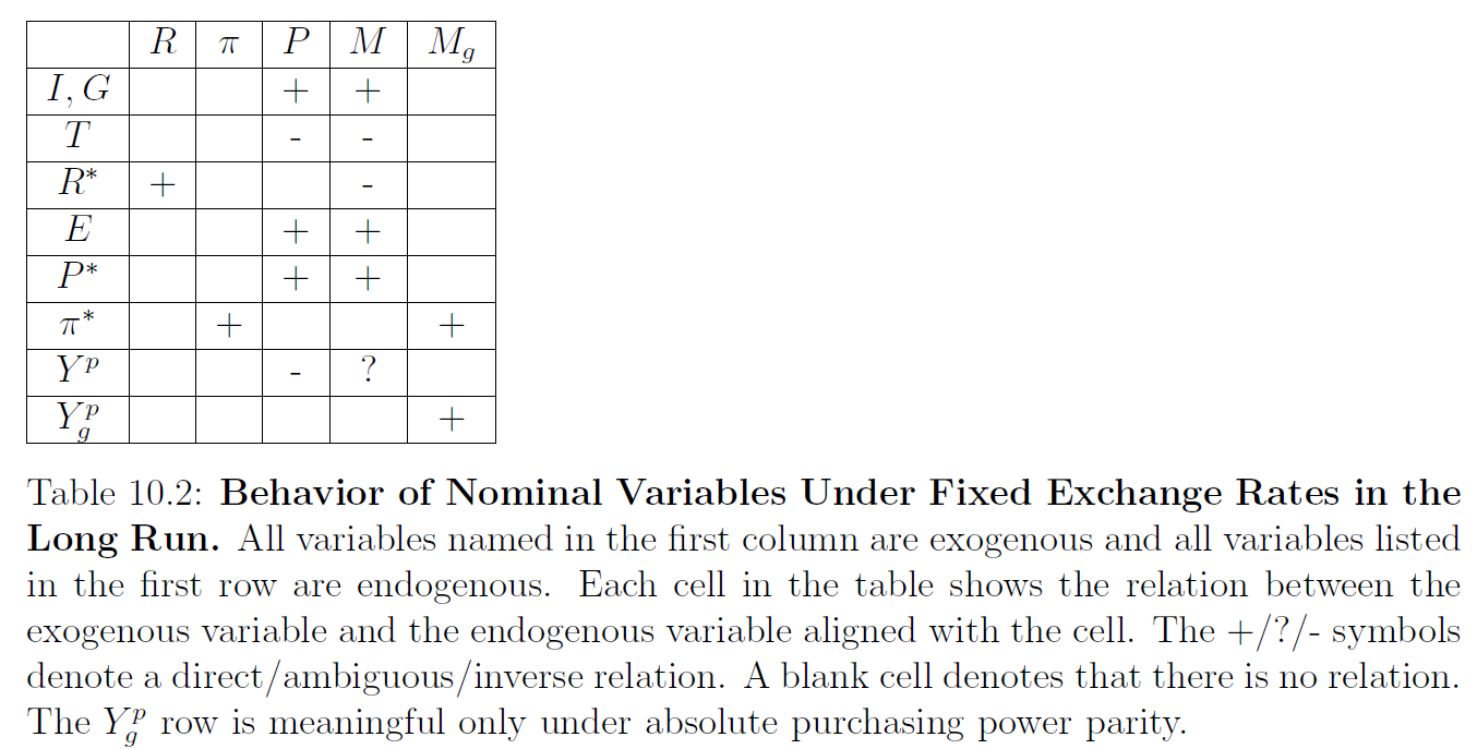
That is, the domestic rate of inflation, $\pi$, is equal to the foreign rate of inflation, $\pi^*$, and unaffected by all other exogenous variables. This is shown in the $\pi$-column of Table 10.2.

10.9.2 The Nominal Interest Rate

Equation 10.4 and Equation 10.13 together imply \[ R=R^*. \tag{10.14}\]

That is, the domestic nominal interest rate, $R$, is equal to the foreign nominal interest rate, $R^*$, and is unaffected by all other exogenous variables. This is shown in the $R$-column of Table 10.2.

Equation 10.13 and Equation 10.14 show how strongly a country gets tied up with the country whose currency its own currency is fixed to. If China fixes the value of its currency, the yuan, to, say, 25 American cents, one yuan would essentially become equivalent to a quarter dollar and the difference between people who carry yuans in their wallets and those who carry dollars would be the same as the difference between those who carry 25 cent coins in their wallets and those who carry one dollar bills. In other words, when the yuan is fixed to the dollar, there is no genuine difference any more between the two currencies, which is why the inflation rates and interest rates in America and China would become equal, just as they are equal in New York and Texas and California.

10.9.3 The Price Level

Equation 4.1, which defines the real exchange rate, can be rewritten as \[ P=\frac {E\cdot P^*}{q}. \tag{10.15}\]

As both $E$ and $P^*$ are exogenous, it follows that the exogenous variables $G$, $I$, $T$, and $Y^p$ will affect $P$ in a way that is precisely the opposite of how Section 9.4 says they affect $q$.

Recall from Section 9.4 that $E$, $R^*$, $\pi^*$ and $P^*$, being nominal variables, do not affect $q$, the real exchange rate. Therefore, Equation 10.15 implies that $P$ is directly affected by $P^*$ and $E$ and unaffected by $R^*$ and $\pi^*$.

To summarize, $P$ is directly affected by $G$, $I$, $P^*$, and $E$, inversely affected by $T$ and $Y^p$ , and unaffected by all other exogenous variables. These ceteris paribus effects are shown in the $P$-column of Table 10.2.

10.9.4 The Quantity of Money

Equation 10.5 and Equation 10.14 together imply: \[ M=L(R^*)\cdot P\cdot Y^p. \tag{10.16}\]

Therefore, for all exogenous variables other than $R^*$ and $Y^p$, their effects on $M$ are the same as what Section 10.9.3 says are their effects on $P$.

According to Section 5.8.4, $L$ decreases when $R(=R^*)$ increases. Moreover, we saw in Section 10.9.3 that an increase in $R^*$ has no effect on $P$. Equation 10.16 then implies that $M$ must decrease when $R^*$ increases.

We also saw in Section 10.9.3 that an increase in $Y^p$ decreases $P$. Therefore, it folows from Equation 10.16 that the effect of an increase in $Y^p$ on $M$ is ambiguous.

To summarize, $M$ is directly affected by $G$, $I$, $P^*$, and $E$; inversely affected by $T$ and $R^*$; ambiguously affected by $Y^p$; and unaffected by all other exogenous variables. These ceteris paribus effects are shown in the $M$-column of Table 10.2.

10.9.5 Growth Rate of the Quantity of Money

Equations Equation 10.6 and Equation 10.13 together imply: \[ M_g=\pi^*+ Y^p_g. \tag{10.17}\]

As both $\pi^*$ and $Y^p_g$ are exogenous, it follows that $M_g$ is directly affected by $\pi^*$ and $Y^p_g$, and unaffected by all other exogenous variables.

This completes my discussion of the long-run behavior of nominal variables in an economy that has a system of fixed exchange rates. The results are summarized in Table 10.2.

10.9.6 The Sustainability of a Fixed Exchange Rate System

Before we end this discussion of long-run international macroeconomics under fixed exchange rates, let us go back to Section 8.1.1 of Chapter 8 and remind ourselves of how a fixed exchange rate system works.

The domestic central bank announces that it is willing to buy/sell currencies at the rate of $\bar{E}$ units of the domestic currency per unit of the foreign currency. Soon after this policy is announced, the market equilibrium value of the foreign currency becomes equal to the domestic central bank’s target rate—$E=\bar{E}$—and the domestic central bank achieves its wish to control $E$.

Unfortunately, as was pointed out in Section 8.1.1, the domestic central bank will no longer be able to exert control over the domestic money supply ($M$), which then becomes an endogenous variable. When people show up at the domestic central bank’s door with bundles of foreign currency and ask for $\bar{E}$ units of the domestic currency for every unit of foreign currency, the domestic central bank will have to print new currency and hand it over to the public. There will, therefore, be a simultaneous increase in the domestic money supply ($M$) and the domestic central bank’s reserves of the foreign currency, which I will denote $F$.

On the other hand, when people approach the domestic central bank, offering $\bar{E}$ units of the domestic currency and seeking one unit of the foreign currency in exchange, the domestic central bank must reach into its foreign currency reserves and hand over the promised amount to the public. Therefore, in this case, there will be a simultaneous decrease in both $M$ and $F$.

In short, in a fixed exchange rate system, domestic money supply ($M$) and domestic reserves of foreign currency ($F$) must move together in lockstep.

This brings us to Section 10.9.4 above. There we saw that the long-run equilibrium value of $M$ could decrease for a number of reasons—for example, decreases in domestic investment ($I$) and/or foreign prices ($P^*$). Now, a money supply decrease of magnitude $\Delta M$ would have to be accompanied by a decrease in foreign currency reserves of magnitude $\Delta F=\Delta M/\bar{E}$. This is because the people will show up at the domestic central bank’s door, hand over $\Delta M$ units of the domestic currency, and ask for $\Delta F$ units of the foreign currency in return.

But what if the central bank just does not have $\Delta F$ units of the foreign currency?

In that case, unless a benevolent foreign government or an international financial institution such as the International Monetary Fund steps in with a loan, the domestic central bank will be forced to take back its promise to exchange $\bar{E}$ units of the domestic currency for each unit of foreign currency. It will have to say, “Sorry, but the deal is off” and put an end to the fixed exchange rate system. The economy would thereafter operate under flexible exchange rates.

Aside from the prospect of being rescued by a foreign-currency loan from a foreign government or the IMF, our discussion in Section 10.9.4 shows another way out: the government can come to the central bank’s rescue and either raise government spending ($G\uparrow$) or cut taxes ($T\downarrow$). As can be checked from the $M$-column of Table 10.2, these policy measures will exert upward pressure on $M$ and, thereby, reverse the initial decline in $M$ that was caused by decreases in $I$ and/or $P^*$. This would remove the threat to the fixed exchange rate system.

However, such expansionary fiscal policies—big increases in government spending and/or big cuts in taxes—will almost surely require deficit financing or, simply, borrowing by the government. And at a time of grave crisis, when the country’s central bank is about to renege on its promise, the credibility of the country’s government may be low and people may not be willing to lend it money. In that case, this country’s fixed exchange rate system would be hard to rescue.

We can learn more about the robustness of a country’s fixed exchange rate system by looking at the long-run equilibrium growth rate of its money supply. This is given in Equation 10.17: $M_g=\pi^*+ Y^p_g$. Although this will most likely be positive, a negative value cannot be ruled out. That would mean continuous and simultaneous decreases in both $M$ and $F$. And, again, if the domestic central bank does not have enough foreign currency reserves to begin with, $F$ could quickly evaporate, in which case the central bank would have to put an end to its fixed exchange rate system.

To summarize the discussion so far, the sustainability of a fixed exchange rate system depends crucially on whether the domestic central bank has a big enough stash of foreign currency. One way for the domestic central bank to ensure this is to adopt what is called a currency board system. In this case the domestic central bank adopts a fixed exchange rate system only when its foreign currency reserves ($F$) are at least $1/\bar{E}$ times the currency held by the public.

To see why this will ensure that the central bank will never run out of foreign currency, let’s try a numerical example. Suppose the amount of domestic currency currenctly held by the public is $10 trillion. Suppose the domestic central bank announces that it is willing to exchange currencies at the rate of $2.00 for : this sets $\bar{E}=2$. If domestic reserves of foreign currency are currently $(1/2)\times 10 =$ trillon, then even if all $10 trillion currently held by the public are brought to the central bank by people clamoring for euros in return, the central bank would still have enough euros to keep its promise. It will not run out of foreign currency reserves.

I will continue my discussion of the sustainability of fixed exchange rate systems and their susceptibility to speculative currency crises in a later chapter.

10.10 Conclusion: Flexible or Fixed?

Now that we have looked at the long-run behavior of nominal economic variables under both flexible and fixed exchange rate systems, which system is better?

A lot comes down to the extent to which a country can neutralize the effects on its economy of things that may be happening in another country.

If it is very important for a country to be able to keep its inflation rate stable and unaffected by economic shocks originating abroad, then a flexible exchange rate system would be preferable. Equation 10.7 shows that $\pi=M_g-Y^p_g$ under a flexible system and Equation 10.13 shows that $\pi=\pi^*$ in a fixed system. Under a fixed exchange rate system, a country’s inflation rate is joined at the hip to the foreign country’s inflation.

On the other hand, under a fixed exchange rate system, the exchange rate is, well, fixed, whereas under a flexible exchange rate system traders engaged in international transactions may have to grapple with a lot of uncertainty over the exchange rate.

In the end, it all comes down to the relative importance of inflation stability versus exchange rate stability for a particular country.

The “classical” in classical dichotomy refers to the classical school of economic thought that was dominant in the eighteenth and nineteenth centuries. Prominent representatives of the classical school include David Hume (1711–1776), Adam Smith (1723–1790), Thomas Malthus (1766–1834), David Ricardo (1772–1823), and John Stuart Mill (1806–1873). The classical dichotomy and the theory of monetary neutrality were central ideas of the classical school and are generally attributed to Hume, although hints of these ideas have been found even in the writings of medieval scholars.↩︎
In case you are wondering where’s Theorem 6.1, please see Section 6.1.3.↩︎
When, in addition, I assume absolute purchasing power parity, I will say so explicitly.↩︎
See Section 5.8.4.↩︎
This is shown in the $\pi$-column of Table 10.1.↩︎