9 Long-Run Predictions: The Real World

What would be the long-run (or, eventual) consequence of an increase in taxes? This and similar other questions are discussed in this chapter and the next. These questions will all have the same format: If there is a permanent increase in [insert the name of an exogenous variable], what will happen in the long run to [insert the name of an endogenous variable]? Notice that the focus will always be on prediction, because only when a theory takes a stand by making a prediction can it be tested with actual data.

We have seen the distinctions between nominal and real gross domestic product— in Chapter 2 — and nominal and real exchange rates—in Chapter 4. Nominal variables are not adjusted for inflation, whereas real variables are. Real variables could meaningfully describe even a barter economy in which money does not exist. Nominal variables, on the other hand, would make sense only in monetary economies. This chapter focuses on the long-run effects of exogenous variables on real endogenous variables. The next chapter takes on nominal endogenous variables, such as the price level, the inflation rate, and the nominal exchange rate.

As I said in Section 7.2, for long-run analysis I will assume:

Full Employment—i.e., $Y = Y^p$—and
Perfect Foresight—i.e., $E^e_f=E_f$.

9.1 Gross Domestic Product

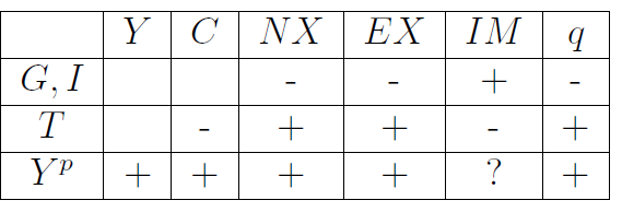
Recall from Section 7.1 that $Y^p$, potential GDP, is, for us, an exogenous variable. Therefore, the full-employment assumption, $Y=Y^p$, says all that can be said about the long-run behavior of GDP: $Y$ is equal to $Y^p$ and unaffected by all other exogenous variables. This is shown in the $Y$-column of Table 9.1, which shows the ceteris paribus effects of each exogenous variable on all endogenous variables.¹

9.2 Consumption

Recall from Equation 5.2 in Section 5.3 that consumption ($C$) is directly related to disposable income ($Y-T$) as in the consumption function, $C=C(Y-T)$. The full-employment assumption that we just saw then implies

\[ C=C(Y^p-T). \tag{9.1}\] As $T$ and $Y^p$ are assumed exogenous for our purposes—see Section 7.1 —we can say right here all that can be said about the long-run behavior of consumption: $C$ is directly affected by $Y^p$, inversely affected by $T$, and unaffected by all other exogenous variables. These are ceteris paribus effects, and they are shown in the $C$-column of Table 9.1.

As consumption is an endogenous variable, we need to be able to explain the ups and downs of $C$. Once we have succeeded in expressing an endogenous variable in terms of exogenous variables alone—as we have done in Equation 9.1 —we can’t go any further because, by definition, exogenous variables are variables we know nothing about (except that they may help explain the up and down movements of our endogenous variables). We don’t know what makes $Y^p$ and $T$ fluctuate. Therefore, once we have expressed $C$ entirely in terms of $Y^p$ and $T$, we cannot say anything more about $C$.

9.3 Net Exports

Recall from Equation 5.8 that $Y=C+I+G+NX$ is the condition that must be satisfied for the goods market to be in equilibrium. Therefore, \[ \begin{eqnarray} NX&=&Y-C(Y-T)-I-G\nonumber \\ &=&Y^p-C(Y^p-T)-I-G \end{eqnarray} \tag{9.2}\] in long-run equilibrium.

Notice that all the variables on the right hand side of this equation are exogenous. Therefore this equation tells us all that can be said about the long run behavior of $NX$.

For example, what if there is a permanent increase in either $I$ or $G$ or both? It follows directly from Equation 9.2 that $NX$ will decrease.

If, however, you are persuaded by the logic of Ricardian equivalence, which we saw in Section 5.3.1, then the analysis would be a lot more subtle. Suppose $G$ has permanently increased by $100 a year. Section 5.3.1 implies that even though the government in this case has not raised taxes to pay for the increased spending, people may behave as if taxes have gone up by the same $100. In that case, $C$ would fall. For a $100 increase in government spending that is perceived to be permanent, $C$ would also fall by $100, the full extent of the perceived/feared increase in $T$ and the actual increase in $G$. And, therefore, the decline in $C$ would cancel out the increase in $G$ in Equation 9.2, leaving $NX$ unchanged.

The effect of an increase in taxes is equally easy to figure out. When $T$ increases, $C$ decreases, as we saw in Section 9.2 above. Therefore, by Equation 9.2, $NX$ will increase.

Finally, what if there is a permanent increase in the domestic country’s potential real GDP ($Y^p$) by, say, $1.00? Consumption spending will increase—as we saw in Section 5.3 above—by the magnitude of the marginal propensity to consume (MPC). And, as we saw in Section 5.3.1, the size of the MPC depends on whether the change in income is perceived to be permanent or temporary. Specifically, if the one-dollar increase in income is perceived to be permanent, $C$ will also rise by one dollar and therefore, by Equation 9.2, $NX$ will be unchanged. But when the one-dollar increase in income is perceived to be less than permanent, $C$ will rise by a fraction of one dollar. So, $Y^p-C(Y^p-T)$ will increase. Therefore, by Equation 9.2, $NX$ will be increase.

So, what’s one to believe? If the permanent increase in $Y^p$ is perceived to be permanent, $NX$ is unaffected by the increase in $Y^p$. But if people doubt the permanence of this increase in $Y^p$, $NX$ increases. It makes sense to split the difference and say that when potential real GDP increases, so does net exports, because in actual cases there may be no increase in potential real GDP that is perceived to be entirely permanent.

To sum up, what does our analysis say about the long-run behavior of a country’s trade balance or net exports? A country’s net exports is directly affected by its potential real GDP and its tax revenues; inversely affected by government spending and investment spending; and unaffected by all other exogenous variables. These are ceteris paribus effects, and they are shown in the $NX$-column of Table 9.1.

9.3.1 Policies to raise net exports

The important lesson of our analysis is that the only dependable way to achieve a long-run increase in net exports is through ‘fiscal austerity’ or ‘belt tightening’ by the country’s government. When government spending is reduced ($G\downarrow$) and/or taxes are raised ($T\uparrow$), net exports increases ($NX\uparrow$).

A surprising related point in that tariffs, which are taxes imposed only on imported goods and services, and other protectionist policies cannot affect a country’s net exports. It would be hard to make a cogent argument that tariffs would lead to an increase in $Y^p$ or in $Y^p-C(Y^p-T)$, or to a decrease in $I$ or in $G$. Therefore, it would be hard to make a persuasive argument that $NX=Y^p-C(Y^p-T)-I-G$ would increase in the long run if tariffs or other protectionist measures are implemented.

9.4 Real Exchange Rate

The analysis of the long-run behavior of the real exchange rate ($q$) depends on whether or not the law of one price is assumed to be true.²

9.4.1 Under absolute purchasing power parity

Recall from Section 5.6.4 that under the law of one price—also called absolute purchasing power parity—the real exchange rate must always be $q=1$ and the relation between net exports and the real exchange rate is represented by a horizontal net exports curve such as the one shown in the right panel of Figure 5.2. In this case, the analysis of the long-run behavior of the real exchange rate is trivial: it will always stay at $q=1$, nothing can make it budge.

Let us, therefore, move on to the less restrictive case shown by the rising net exports curve in the left panel of Figure 5.2.

Figure 9.1: This diagram shows how real exchange rates can change. In long-run equilibrium, both $NX=NX(q,Y^p-T)$ and $NX=Y^p-C(Y^p-T)-I-G$ must be true. Therefore, for the initial values $Y^p=Y^p_0$ and $T=T_0$, the equilibrium is at point $A$. When either $T$ increases or $Y^p$ decreases, the upward-sloping net exports curve shifts right, as shown. When $T$ increases, the vertical net exports curve also shifts right, but by more than the upward-sloping net exports curve does. As a result, the long run equilibrium moves from $A$ to $C$. This implies a direct effect of $T$ on $q$. When $Y^p$ decreases, the vertical net exports curve shifts left. As a result, the long run equilibrium moves from $A$ to $E$. This implies a direct effect of $Y^p$ on $q$; they both move in the same direction. When either $I$ or $G$ increases, the upward-sloping net exports curve is unaffected and the vertical net exports curve shifts left, taking the equilibrium from $A$ to $D$. This shows that $I$ and $G$ have inverse effects on $q$. No other exogenous variable affects $q$. (Note that absolute purchasing power parity has *not* been assumed.)

9.4.2 Without absolute purchasing power parity

9.4.2.1 Two net exports curves: one upward-sloping, the other vertical

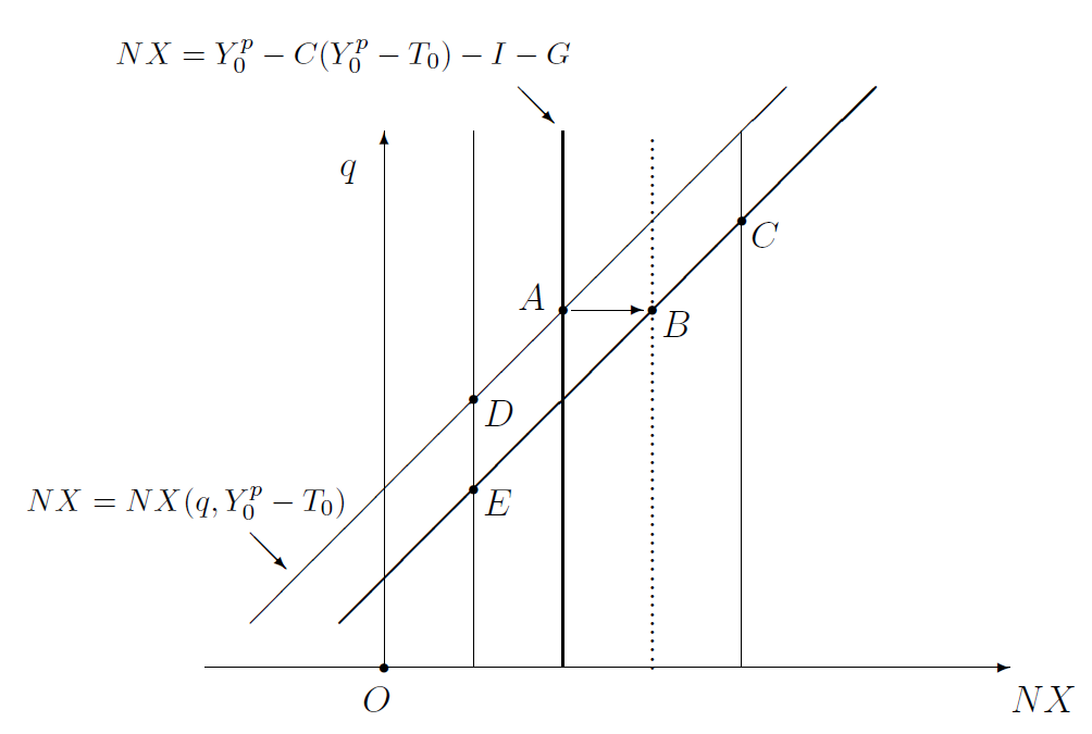
Recall from Equation 5.6 that $NX=NX(q,Y-T)$ is directly related to $q$ and inversely related to $Y-T$. For some given value of $Y-T$, the direct effect of $q$ on $NX$ is shown as an upward-sloping net exports curve in the left panels of Figure 5.2 and Figure 5.3 and yet again in Figure 9.1 in this chapter.³

These figures also show that a decrease in $Y^p$ or an increase in $T$ or, generally, a decrease in $Y-T=Y^p-T$ shifts the upward-sloping net exports curve downward or to the right. A poorer country imports less and, therefore, sees its net exports increase at any given value of the real exchange rate.

In fact, we can be more specific about the size of this shift. Recall from Section 5.6.2 that if $Y-T$ decreases by a dollar, both consumption ($C$) and imports ($IM$) will decrease, but the latter will decrease less than the former. In particular, $C$ decreases by the marginal propensity to consume (MPC) and $IM$ decreases by less than the MPC. It therefore follows that when $Y^p-T$ decreases by a dollar, $NX$ will increase by less than the MPC, at any given value of the real exchange rate. In other words, when $Y^p-T$ decreases by a dollar, the vertical net exports curve shifts right by a length smaller than the MPC.

Now, as we saw in Section 9.3 above, the goods market’s equilibrium condition, $Y=C+I+G+NX$, also tells us something about a country’s net exports. Specifically, $NX=Y-C(Y-T)-I-G$ or, in long-run equilibrium, $NX=Y^p-C(Y^p-T)-I-G$. As this equation expresses $NX$ as entirely independent of $q$, it can be graphically shown as the vertical net exports curve in Figure 9.1. It is vertical because changes in $q$ have no effect on $NX=Y^p-C(Y^p-T)-I-G$. Of course, if $Y^p$ or $T$ or $I$ or $G$ changes in value, so will $NX$ and the vertical net exports curve will shift.

For example, if either $I$ or $G$ increases by a dollar, $NX=Y^p-C(Y^p-T)-I-G$ will decrease by a dollar and the vertical net exports curve will shift left by a dollar. If $T$ increases by a dollar, $C$ will decrease, not by the entire dollar’s increase in taxes but by a fraction—a fraction that was called the marginal propensity to consume (MPC) in Section 5.3.1. As a result, $NX=Y^p-C(Y^p-T)-I-G$ will increase by that same amount (the MPC). Therefore, when $T$ increases by a dollar, the vertical net exports curve shifts right by a length equal to the MPC.

Finally, if $Y^p$ increases by a dollar, then $C(Y^p-T)$ increases by the MPC. Therefore, $Y^p-C(Y^p-T)$, which is simply the part of total income that is saved, will increase by $1-\text{MPC}$ dollars, which is equivalent to MPS dollars, where MPS stands for the marginal propensity to save—see Section 5.3.1. In short, when $Y^p$ increases by a dollar, the vertical net exports curve shifts right by MPS dollars.

9.4.2.2 Equilibrium

Now, in long-run equilibrium, what we know about the factors that influence net exports ($NX=NX(q,Y^p-T)$, the upward-sloping net exports curve) must be consistent with what the goods market’s equilibrium condition tells us about net exports ($NX=Y^p-C(Y^p-T)-I-G$, the vertical net exports curve). Therefore, in Figure 9.1, the long-run equilibrium must be at $A$, where the two net exports curves intersect. This pinpoints the long-run equilibrium level of the real exchange rate.

And, as we know how the two net exports curve shift when there are changes in the magnitudes of the exogenous variables $Y^p$, $T$, $I$, and $G$, we will be able to predict how the real exchange rate is affected by these changes.

For example, as we saw in the previous section, if either $I$ or $G$ increases, the upward-sloping net exports curve is unaffected and the vertical net exports curve shifts left. Therefore, the long-run equilibrium in Figure 9.1 moves from $A$ to $D$, implying a decrease in $q$. That is, increases in domestic spending either by businesses ($I\uparrow$) or the government ($G\uparrow$) boosts the relative demand for the domestic country’s products and thereby raises the relative price of those products or, equivalently, reduces the relative price of foreign goods ($q\downarrow$).

We have also seen that if $T$ increases by a dollar, the upward-sloping net exports curve shifts right by less than the MPC. On the other hand, we have also seen that the vertical net exports curve shifts right by a length equal to the MPC. Therefore, the long-run equilibrium in Figure 9.1 will move from $A$ to $C$, implying an increase in $q$. That is, an increase in taxes ($T\uparrow$) leads to a higher real exchange rate ($q\uparrow$). This is intuitive: A rise in taxes squeezes domestic consumption, which reduces demand in the domestic economy. This reduces the relative price of domestic goods or, equivalently, raises the relative price of foreign-made goods, which is the real exchange rate.

Finally, we have seen in the previous section that if $Y^p$ decreases by a dollar, the upward-sloping net exports curve shifts right and the vertical net exports curve shifts left. Therefore, the long-run equilibrium in Figure 9.1 moves from $A$ to $E$, implying a decrease in $q$. That is, as in the case of $T$, a change in $Y^p$ brings about a change in $q$ in the same direction.

And, again, this is intuitive. If a country becomes more productive ($Y^p\uparrow$) its goods become relatively more plentiful in the world economy. This drives down the relative price of domestic goods or, equivalently, makes foreign-made goods relatively more expensive ($q\uparrow$).

9.4.2.3 Real Exchange Rate: Summary

To summarize, under absolute purchasing power parity, $q=1$ in all situations and is, therefore, unaffected by changes in our exogenous variables. When absolute purchasing power parity is not applicable, in long run equilibrium, the real exchange rate ($q$) is inversely affected by government spending ($G$) and business investment ($I$); directly affected by taxes ($T$) and potential output ($Y^p$); and unaffected by all other exogenous variables. These ceteris paribus effects are shown in the $q$-column of Table 9.1.

In Chapter 10, a less stringent version of absolute purchasing power parity—called relative purchasing power parity—is assumed. Relative purchasing power parity is the assumption that the real exchange rate is constant over time, though not necessarily equal to one—see Section 10.4. Given the results summarized in the previous paragraph, for the real exchange rate to be constant, either $I$, $G$, $T$, and $Y^p$ would have to be constant or—and this is an unlikely possibility—they would have to change in concert in such a way that they cancel each others’ effects on $q$ and, therefore, leave the real exchange rate constant.

Table 9.1: **Macroeconomic Behavior of Real Variables in the Long Run**. All variables named in the first column are exogenous and all variables listed in the first row are endogenous. Each cell in the table shows the relation between the exogenous variable and the endogenous variable aligned with the cell. The +/?/- symbols denote a direct/ambiguous/inverse relation. A blank cell denotes that there is no relation. Note that absolute purchasing power parity has *not been assumed. Under APPP, the last three columns would be gone and the rest of the table would be unaffected. Recall that $q$ is constant at $q=1$ under APPP. Moreover, the $EX$ and $IM$ columns would be gone too, as they would no longer make sense, being infinitely elastic at $q=1$.

9.5 Exports

Recall from Equation 5.4 in Section 5.6.1 that the amount of domestically produced goods that is exported ($EX=EX(q)$), is directly related to the real exchange rate ($q$).⁴

Therefore, if an exogenous variable has a direct/non-existent/inverse effect on $q$ it will have an identical effect on $EX$. In Table 9.1, therefore, the $EX$-column must necessarily be the same as the $q$-column that was discussed in Section 9.4 above.

9.6 Imports

Recall from Equation 5.5 in Section 5.6.2 that the amount imported by a country in the long run ($IM=IM(q,Y^p-T)$) is inversely related to the real exchange rate ($q$) and directly related to the disposable potential real GDP ($Y^p-T$).

According to Section 9.4, a ceteris paribus increase in $G$ or $I$ causes a decrease $q$. This, in turn, would increase $IM$.

An increase in $Y^p$ leads to a higher $q$, which reduces imports, and a higher $Y^p-T$, which increases imports. Therefore, the overall effect of $Y^p$ on $IM$ is ambiguous.

An increase in $T$ leads to an increase in $q$ and a decrease in $Y^p-T$. Both lead to reduced imports.

To summarize, imports are directly affected by $G$ and $I$; inversely affected by $T$; ambiguously affected by $Y^p$; and unaffected by all other exogenous variables.

9.7 Macroeconomic Behavior of Real Variables in the Long Run: Conclusions

We have been discussing the long-run effects of our exogenous variables on our real endogenous variables. The results are summarized in Table 9.1.

Note that only fiscal policy can affect net exports; tariffs, for example, are useless. Contractionary fiscal policy—i.e., either a cut in government spending, $G$, or an increase in taxes, $T$, or both—can reliably increase net exports.

Note also that neither monetary variables—such as $M$, $P$, and $E$—nor the money market equilibrium condition—that is $M=L(R)\cdot P\cdot Y$ in Section 5.8.5 —played any role in this chapter’s discussion of the long run behavior of real variables. In fact, I did not even mention any monetary variables before this paragraph. This is an instance of an idea with a long pedigree in economics called monetary neutrality: any change in the quantity of money in circulation ($M$) will not affect a real variable.

While monetary neutrality is thought to be a good description of an economy in the long run, we will see that things are different in the short run. In the short run, $M$ can be an important determinant of real variables such as $Y$, $C$, $I$, $q$, and $NX$.

Note, finally, that in this chapter I did not bring up the issue of whether the country has a flexible exchange rate system or a fixed exchange rate system. In other words, the exchange rate system has nothing to do with the long run behavior of real variables. Put yet another way, the long run analysis of real variables will have nothing useful to say if a country is debating what kind of exchange rate system to adopt: both systems have the same real consequences.

See Section 6.2 for the definition of ceteris paribus effects.↩︎
See Section 4.2 for more on the real exchange rate, and Section 5.6.3 and Section 5.6.4 for more on the law of one price.↩︎
Figure 9.1 also makes use of the long-run assumption of $Y=Y^p$. The upward-rising net exports curve marked with a label and an arrow assumes that the magnitude of potential output is $Y^p=Y^p_0$ and the magnitude of taxes is $T=T_0$.↩︎
For a recap on real exchange rates, see Section 4.2.↩︎