5 Markets and Equilibrium

A theory that says “Anything is possible” or “All conceivable outcomes are equally plausible” would not be of any use. To be useful, a theory must put its foot down and take a stand on which outcomes are plausible and which outcomes are not. For an outcome to be considered plausible, the typical theory in economics requires that all relevant markets (for goods, services, and assets) be in equilibrium, which is when supply and demand are equal. This chapter describes the conditions that must prevail in the markets for goods, money, and foreign currency for them to be in equilibrium.

5.1 The Goods Market Equilibrium Condition

The goods market is said to be in equilibrium when

\[ Y=C+I+G+NX. \tag{5.1}\]

You have seen this equation before as Equation 2.5 or the national income identity of Section 2.5. However, Equation 5.1 is actually quite different from Equation 2.5, in the sense that $Y$, $C$, $I$, $G$, and $NX$ are defined differently in these two equations.

In Equation 2.5, the five symbols were defined in such a way that $Y$ had to be equal to $C+I+G+NX$ simply by virtue of the definitions of the five symbols. In Section 2.5, $Y$, $C$, $I$, $G$, and $NX$ were defined as the actual magnitudes of gross domestic product, personal consumption expenditures, gross private domestic investment, government spending, and net exports of goods and services that are published periodically by government statisticians. And, as we saw in Section 2.5, under those definitions, $Y$ had to be equal to $C+I+G+NX$.¹

In Equation 5.1, on the other hand, $Y$ represents the output that domestic producers wish to produce (supply) and $C+I+G+NX$ now represents the total purchases of domestically produced goods and services desired by buyers the world over (demand). Therefore, $Y$ and $C+I+G+NX$, as redefined for Equation 5.1, are not necessarily equal. When they are equal, we say that the goods market is in equilibrium.

As you will see later, the goods market equilibrium condition—as well as the other equilibrium conditions that I will discuss later—helps to rule out certain economic outcomes. As a result, our theory will be able to make predictions that are specific and not say something vague and useless such as “Anything is possible”.

5.1.1 Components of Aggregate Expenditure

The total purchases of domestically produced goods and services desired by buyers the world over—that is, the demand for “Made in USA” goods and services—is referred to as aggregate expenditure. In parallel to the discussion of the components of gross domestic product in Section 2.4, we can specify the components of aggregate expenditure.

$Y$ is the real (i.e., inflation-adjusted) value of the total output that the firms of the country we are analyzing—the domestic country—would like to produce. That is, $Y$ is what the gross domestic product would be if the firms’ production levels turn out to be what they had planned.
Since our incomes are what we get for the work we do, $Y$ is also the total income of the domestic country’s households. (It should be clear that if a firm’s output—or value added, to use a technical term—was $500,000 in 1999, that amount must have ended up as the incomes of the households that owned the resources used by the firm.)
$C$ is the real consumption spending desired by residents of the domestic country.
$I$ is the real investment expenditure that the firms in the domestic country would like to make.
$G$ is the real level of spending planned by the domestic country’s government.
$NX$ is the real net exports of the domestic economy that would result from the plans of all exporters and importers.

5.1.2 What Does the Goods Market Equilibrium Condition Mean?

Note that we have $Y$, the supply of “Made in USA” goods, on the left hand side of Equation 5.1. Therefore, for Equation 5.1 to represent equilibrium, the right hand side ought to be the demand for “Made in USA” goods. But is it?

Let’s look at the people who buy “Made in USA” goods. Such goods are bought by

American households, for consumption
American businesses, for investment
the U.S. government, for government spending, and
foreigners, as our exports

Therefore, it would seem that the demand for “Made in USA” goods is simply $C+I+G+\text{Exports}$. But wait! $C$ includes consumption spending on French wine, Italian cheese, etc. $I$ includes investment spending on German machine tools and Korean earth-moving equipment. And $G$ includes government spending on British-made Jaguar cars. Therefore, to calculate the demand for “Made in USA” goods, one must deduct Imports from $C+I+G+\text{Exports}$. That is, the demand for “Made in USA” goods is given by $C+I+G+\text{Exports}-\text{Imports}$ or $C+I+G+NX$, which is precisely what’s on the right hand side of Equation 5.1.

Therefore, we see that Equation 5.1 does indeed represent equilibrium in the goods market.²

As we saw in the previous section, the demand for domestically produced goods, $C+I+G+NX$, is also referred to as aggregate expenditure ($AE$). Consequently, the goods market equilibrium condition can be written compactly as $Y=AE$.

5.1.3 What’s the Use of an Equilibrium Condition?

When the variables in the goods market equilibrium condition, Equation 5.1, are interpreted as in the statistical tables of the United States’ National Income and Product Accounts, it becomes an identity that is useless for theoretical purposes because identities are always true by definition. The definitions in Section 5.1.1 on the other hand interpret the variables as plans or desired levels. Therefore, $Y$ can be thought of as the supply of ‘Made in USA’ goods and the expression on the right hand side of Equation 5.1 can be interpreted as the demand for ‘Made in USA’ goods. Therefore, the goods market equilibrium condition may be seen as another form of the familiar “supply equals demand” idea.

To repeat the discussion at the beginning of Section 5.1, unlike Equation 2.5, which is an identity and, therefore, always true by definition, Equation 5.1 is true only under pretty unique circumstances and for pretty unique magnitudes of the variables in the equation. Without equations like the one above, it would be an “anything goes” situation and any useful analysis would be impossible. The equation above asserts, “Only those values of $Y$, $C$, $I$, $G$ and $NX$ that obey the equation will prevail in reality.” So, equations like the one above will allow us to be specific about the conditions under which certain important variables, such as $Y$, may increase or decrease.

5.2 Notation: Functional Relationships

Before we go any further with our analysis, we need to discuss a notation-related issue.

If a variable $y$ is related in some way to a variable $x$, we denote this as $y=f(x)$. There is nothing special about the letter $f$ in the equation: any other letter (or letters) would have done just as well. The key point is that the variable that represents the cause—in this case $x$—is put within parentheses and the variable that represents the effect—in this case $y$—is put on the left of the equals sign. Saying $y=f(x)$ amounts to saying that $y$ depends on $x$.

Similarly, if a variable $z$ is related to the variables $x$ and $y$, we denote this as $z=f(x,y)$.

To avoid confusion, when a dot is placed in front of the opening parenthesis—that is, when I write “$\cdot($”—no functional relation is implied. For example, in the equation $w=x\cdot(y-z)$, there is no functional relationship implied. All it says is that $w$ is equal to the product of $x$ and $y - z$.

5.3 What Are the Factors that Affect Consumption?

The consumption plans of households will be assumed to satisfy the following equation, which is called the consumption function:

\[ C=C(Y-T). \tag{5.2}\]

As we saw in Section 1.4.1, the symbol $T$ denotes the government’s total tax revenues. Therefore, $Y-T$ is the disposable (or after-tax) income of households. Equation 5.2 uses functional notation—see Section 5.2 above—to say that planned consumption spending depends on disposable income.³ More specifically, we assume that consumption is directly related to disposable income: $C$ increases (respectively, decreases) when $Y-T$ increases (respectively, decreases).

Figure 5.1: **Consumption Function**. The solid line shows the relation between consuption spending ($C$) and income ($Y$) for some specified level of taxes ($T$). Note that an increase in $Y$ from $1.00 to $2.00 causes $C$ to increase from $2.67 to $3.33. (Don’t be alarmed: $C$ can exceed $Y$ when people dis-save (or, borrow) to spend more than what they earn.) In other words, when $Y$ increases by $1.00, $C$ increases by $0.67, indicating that $\hbox{MPC}=0.67$. When $T$ increases by $1.00, $C$ decreases—at every level of $Y$—by the same $0.67. That is, an increase in $T$ causes the entire consumption function to shift downwards to the dotted line.

This does not mean that consumption is assumed to change only when disposable income changes. Other factors may also affect consumption. For example, if home prices—or, generally speaking, asset prices, such as the prices of the stocks and bonds and real estate owned by households—increase, people may feel wealthy and, as a result, begin to save less and consume more. Changes in interest rates may also affect the desire to save and the urge to consume. Equation 5.2 merely simplifies the story, highlights the role of disposable income, and downplays the effect of asste prices, interest rates, and other variables on consumption spending.

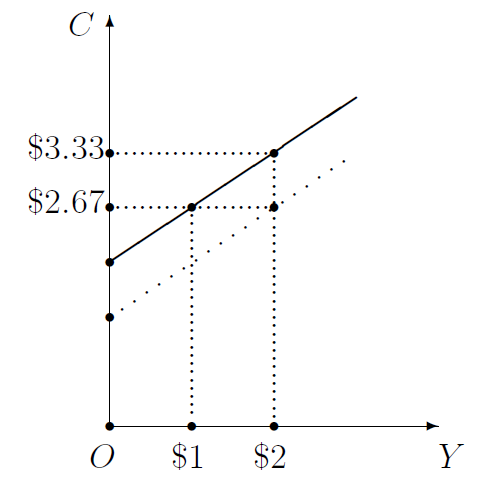
The effect of income and taxes on consumption is graphically shown in Figure 5.1. Assuming taxes ($T$) are unchanged, an increase in income ($Y$) implies an increase in disposable income ($Y-T$) and, therefore, an increase in consumption ($C$), as shown by the solid line in the figure. On the other hand, an increase in $T$ implies a decrease in $Y-T$ at any specified level of $Y$. Therefore, $C$ decreases at every $Y$, implying a downward shift of the consumption function, to the dotted line in Figure 5.1.

5.3.1 The Marginal Propensity to Consume and Ricardian Equivalence

An important point to note about the consumption function is that it is often not enough to make the qualitative statement that increases in disposable income lead to increases in consumption spending: the quantitative magnitude of the effect can be important as well. One could ask, “If disposable income ($Y-T$) increases by one dollar (and if all the other factors that affect consumption spending—such as the asset prices and interest rates mentioned in the last paragraph—remain unchanged), by how many dollars will consumption increase?”

The answer to this question is the marginal propensity to consume. For example, if people spend 70 cents out of every dollar of additional disposable income and save the remaining 30 cents, we say that the marginal propensity to consume (MPC) is 0.70 and the marginal propensity to save (MPS) is 0.30.⁴

In Figure 5.1, for example, the MPC is 0.67. As a result, when $Y$ increases by $1.00, $C$ increases by $0.67. In general, when $Y$ increases (respectively, decreases) by $$x$, $C$ increases (respectively, decreases) by $0.67$x$. On the other hand, a one-dollar increase in $T$ implies a one-dollar decrease in disposable income, causing $C$ to decrease by $0.67 at every value of $Y$. As a result, the consumption function shifts downward by the amount of the MPC when taxes increase by one dollar. In general, when $T$ increases (respectively, decreases) by $$y$, the consumption function shifts down (respectively, up) by $0.67$y$.

It is typically assumed that the magnitude of the MPC depends on whether a change in disposable income is perceived to be permanent or temporary. If the income of a household increases by $500 a month and if this is perceived to be a permanent increase, it is reasonable to assume that consumption spending will also increase by nearly $500 a month. In other words, for changes in $Y$ or $T$ that are perceived to be permanent, it is reasonable to assume $\text{MPC}=1$ and $\text{MPS}=0$. On the other hand, if the people receive a tax cut in the run-up to an election and come to believe that the tax cut will be revoked once the election is over, then it is reasonable to assume that the people will save the bonanza from the tax cut. In other words, for changes in $Y$ or $T$ that are perceived to be temporary, it is reasonable to assume $\text{MPC}=0$ and $\text{MPS}=1$.⁵

People’s estimation of the permanence of a tax cut may also depend on whether the tax cut is accompanied by a cut in government spending, $G$. If there is a cut in taxes but none in government spending, the government would have to borrow from private lenders (for example, banks) to make up the shortfall in tax revenue. But the borrowed money would eventually have to be repayed—with interest. Where would the government get the money to do so? It would probably raise taxes.⁶ Therefore, if people are smart enough, they may come to believe that a tax cut unaccompanied by a cut in government spending is very likely a temporary tax cut that would lead eventually to a tax hike larger than the tax cut itself. They may therefore respond to the tax cut, not by going on a shopping spree, but instead by socking the tax cut away in a bank thinking that a big tax increase is on the way.

This sceptical view of the effect of a tax cut on consumption spending is referred to as the theory of Ricardian equivalence. Let’s consider this further with a numerical example. Suppose the government reduces taxes ($T$) from $1000 to $900 but leaves annual government spending ($G$) unchanged at $1000. The government borrows $100 from a bank at a 7% interest rate to make up the shortfall in tax revenue. Therefore, a year later the government would have to repay $107 to the bank. Therefore, people may conclude that the $100 tax cut is illusory and would inevitably be followed by a $107 tax increase a year later—to the level of $1107 to pay for $1000 in government spending plus $107 in loan repayment. Knowing that they would need an extra $107 next year, what would the people do? They would take the $100 tax cut and put it in a bank so that, at 7% interest, they would have enough next year to pay the tax hike they know is coming.

In other words, when a reduction in $T$ is not accompanied by an equal cut in $G$, $\hbox{MPC}=0$ and $\hbox{MPS}=1$.

Another implication of the theory of Ricardian equivalence is that in some circumstances consumption spending may respond as if taxes have changed even if they actually haven’t! Let’s say government spending increases by $100 but taxes stay the same. Once again, the government would have to borrow $100 from a bank. Therefore, a year later it would need to raise taxes by $107 (assuming 7% interest, as before) to repay the loan with interest. Therefore, taxes would have to rise next year by $107. Therefore, if people anticipate all this, they would put away an extra $100 in their bank accounts in preparation for the $107 tax increase they can see coming. In other words, if $G$ increases and $Y-T$ remains unchanged, $C$ would fall, as if the people are saying to themselves that taxes have risen even though they actually have not.

Therefore, according to Ricardian equivalence, when analysing the effect of a change in government spending it might be a good idea to pretend that the change in $G$ is accompanied by an equal change in $T$, even if $T$ is actually unchanged.

5.4 What Are the Factors that Affect Investment?

Unlike consumption spending ($C$), which has been assumed above to depend on disposable income ($Y-T$), the total of the investment plans of businesses ($I$) is assumed, for simplicity, to dance to its own tune, to be unrelated to other economic variables.

To use a term that will be explained in Section 6.1.1, investment will be assumed here to be an exogenous variable. You will see later that fluctuations in $I$ can explain fluctuations in other variables such as $Y$. But you will see no explanation of the fluctuations in $I$ itself. Investment will be used here as an explanatory variable, but it will remain unexplained itself.

In a theory that argues that increases in temperature cause increases in murder rates, but has nothing to say about what causes temperature to increase, temperature is exogenous and the murder rate is endogenous. In this case, the author of the theory may be admitting that the weather is too complex to explain. Or, perhaps she has concluded that trying to explain the weather would be a waste of time: as we cannot control the weather, it would make sense to forget about what causes temperature fluctuations and instead concentrate on how to deploy the police strategically on hot days to keep murder rates from spiking. Either way, weather is being treated as exogenous.

Returning to the issue at hand, investment is actually not entirely mysterious. A strong case can be made that $I$ depends on the real (or, inflation-adjusted) interest rate, which is the inflation-adjusted cost of the money that businesses need to borrow in order to pay for their investment spending.⁷

Advances in technology and increases in the quantity and quality of a nation’s work force are important influences too. When such changes happen, the productivity of capital goods (such as equipment, machinery, software, etc.) increases. This induces greater investment in additional capital goods.⁸

That said, most economists agree that investment spending by businesses is overwhelmingly dependent on that elusive thing called the optimism or the “animal spirits” of businesspeople. And, as business psychology is not their strong suite, economists tend not to say much about such things. I will simply assume that the level of investment is exogenous or inexplicable—it is what it is.

5.5 What Are the Factors that Affect Government Spending?

Who knows?! Ask your Poli-Sci professor. I will treat $G$ as a variable that is inexplicable but nonetheless useful in explaining changes in other variables such as $Y$, $C$, $NX$, etc. In other words, I will consider $G$ to be exogenous—see Section 6.1.1.⁹

5.6 What Are the Factors that Affect Net Exports?

As we saw in Section 2.4.4 and Section 5.1.1, net exports is the excess of exports over imports: \[ NX\equiv EX-IM, \tag{5.3}\] where, $EX$ denotes the real (i.e., inflation-adjusted) value of the planned sales of domestically produced goods and services to foreign residents, and $IM$ denotes the real value of the demand for foreign-made goods from domestic residents. Therefore, to understand what drives $NX$ up and down, we need to look at what makes $EX$ and $IM$ fluctuate.

5.6.1 What Are the Factors that Affect Exports?

I will assume that the demand from foreign residents for the goods and services produced in the domestic economy—i.e., the domestic country’s exports—is given by

\[ EX=EX(q), \tag{5.4}\] where, as was pointed out in Section 4.2, the real exchange rate ($q$) is the amount of domestically produced goods that can be obtained in trade for one unit of foreign-made goods. As the real exchange rate is the relative price of foreign goods (in units of domestic goods), a rise in $q$ would encourage foreigners to buy more domestic goods. That is, $EX$ and $q$ are directly related.

The real exchange rate, however, is not the only thing that affects exports. An important influence is foreign GDP. For example, countries such as China, Japan, and Germany saw sharp declines in their exports to the US during the US recession of 2008–09. To keep things simple, however, I will ignore this issue and assume that $EX$ depends on $q$ alone.

5.6.2 What Are the Factors that Affect Imports?

I will assume that the domestic country’s demand for foreign-made goods—i.e., its imports—is given by

\[ IM=IM(q,Y-T). \tag{5.5}\]

Since the real exchange rate, $q$, is the amount of domestically produced goods that can be obtained in trade for one unit of foreign-made goods, it should be clear that a high level of $q$ would discourage the import of foreign-made goods; i.e., $q$ and $IM$ are inversely related.

And, as we saw in Section 5.3 above, increases in disposable income ($Y-T$) lead to increases in consumption spending ($C$). Part of this additional consumption is likely to consist of foreign-made goods. Therefore, it follows in an obvious way that $Y-T$ and $IM$ are directly related. Moreover, it also follows that when disposable income increases, consumption increases more than imports do. That is, the marginal propensity to import is smaller than the marginal propensity to consume.

It is also important to keep in mind that just as the effect of a change in disposable income on consumption spending depends on whether the change in disposable income is perceived to be permanent or temporary—see Section 5.3.1 for a reminder—so does the effect of a change in disposable income on households’ purchases of imported goods.

5.6.3 Summary: What Are the Factors that Affect Net Exports?

Section 5.6.1 and Section 5.6.2 imply that we can summarize the nature of a country’s net exports by the equation

\[ NX=NX(q,Y-T). \tag{5.6}\]

Moreover, we can conclude that net exports ($NX$) is related directly to the real exchange rate ($q$) and inversely to disposable income ($Y-T$).

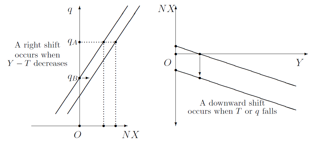
These effects of $q$, $Y$, and $T$ on $NX$ are shown graphically in the two panels of figure Figure 5.2. The left panel emphasizes the role of the real exchange rate in a nation’s net exports. This rising net exports curve shifts rightward when $Y-T$ decreases, indicating lower imports and, therefore, higher net exports at every value of $q$. The right panel of figure Figure 5.2, on the other hand, emphasizes the role of GDP in determining a nation’s net exports. This net exports curve is negatively sloped, indicating that rising incomes lead to rising imports and, therefore, falling net exports. Both graphical representations of $NX$ in figure Figure 5.2 are useful, depending on the context.

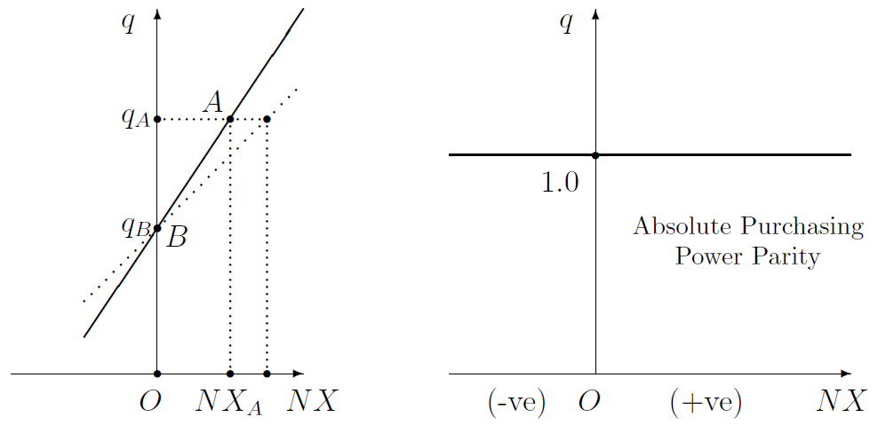
Figure 5.2: **Net Exports** This figure shows that both the real exchange rate ($q$) and taxes ($T$) have a direct effect on net exports ($NX$) and that GDP ($Y$) has an inverse effect. The left panel highlights the effect of the real exchange rate. This curve shifts right when $Y-T$ decreases. The right panel highlights the effect of real GDP. This curve shifts down when either $q$ or $T$ decreases. Note that net exports could be positive or negative. Absolute purchasing power parity is *not* assumed for this diagram.

The direct relation between $NX$ and $q$ is shown one more time in figure Figure 5.3. The left panel in particular shows that as $q$ increases from $q_B$ to $q_A$, $NX$ increases from $NX=0$ to $NX=NX_A$. Had the net exports curve instead been the flatter dotted line, the same change in the real exchange rate would have provoked a bigger change in net exports. In other words, the flatter the net exports curve is—or, the more elastic it is, if you can forgive the jargon—the more responsive $NX$ is to $q$. In the extreme case of infinite responsiveness or elasticity, the net exports curve is horizontal.

If, moreover, the net exports curve is horizontal at $q=1$, as in the right panel of figure Figure 5.3, it is said to obey the law of one price or absolute purchasing power parity. This is discussed further in the next section.

Figure 5.3: **Net Exports and the Real Exchange Rate** The left panel shows a general direct relation between net exports and the real exchange rate. Note that net exports could be positive or negative. The right panel shows the relation between net exports and the real exchange rate under the law of one price or, equivalently, under absolute purchasing power parity.

5.6.4 The Law of One Price and Purchasing Power Parity

The direct relation between net exports and the real exchange rate, when taken to an extreme, leads to the law of one price or, equivalently, absolute purchasing power parity (PPP). This requires that net exports be infinitely elastic with respect to changes in the real exchange rate ($q$) and that

\[ q\equiv\frac{E\cdot P^*}{P}=1. \tag{5.7}\]

The first equality in Equation 5.7 is simply the algebraic definition of the real exchange rate that we saw in Equation 4.1 of Section 4.2. What is new in Equation 5.7 is its insistence that $q=1$.

To see the logic behind this, let us work through an example. Suppose the price, $P$, of American wheat is 2 dollars per pound; the price, $P^*$, of French wheat is 3 euros per pound; and the price of a euro, $E$, is $2.00. Therefore, the price of French wheat in US dollars is $E\times P^*=2.00\times 3=6$ US dollars, thrice the price of identical US wheat.

How likely is this situation—in which the real exchange rate is $q=2.00\times 3/2=3$—to persist? Not very likely, is the clear answer. People all over the world will see a juicy opportunity for arbitrage , which is a fancy term for the practice of making money by buying something at a cheap price and selling it at a higher price. People will start buying American wheat to sell in France. As long as $q=3$ persists, nobody will wish to sell wheat in the US and everybody will want to make money by buying up every grain of US wheat and selling it in France. This is clearly unsustainable. Net exports from America to France will be literally infinite!

On the other hand, suppose $P=2$ dollars per pound of American wheat, as before; $E=2.00$ dollars per euro, also as before; but $P^*=0.50$ euros per pound of French wheat. Now the price of French wheat in dollars is $E\times P^*=2.00\times 0.50=1$ dollar, half the price of identical American wheat.

How likely is this situation—in which the real exchange rate is $q=2.00\times 0.50/2.00=0.50$—to persist? Again, not very likely. People will now wish to buy every grain of French wheat for sale in America. Net exports from America to France will now be negative infinity, which is clearly an unsustainable situation.

For planned net exports to be neither infinity nor negative infinity, the price of wheat must be equal in America and France (when both prices are measured in the same currency). This is the basic idea of the law of one price: the price of any tradable commodity, when measured with the same yardstick, should be the same everywhere if there are no trade-related costs.

To be specific, note that when I calculated the price of French wheat in dollars in the numerical examples above, I multiplied $E$ and $P^*$. Therefore, saying that the price of wheat, when measured in the same currency, should be the same in America and France amounts to saying that \[ E\cdot P^* = P, \] which in turn implies $q=1$ or absolute purchasing power parity, as in Equation 5.7.

Note also that as the magnitude of America’s net exports is infinity when American goods are cheaper than French goods ($q>1$) and negative infinity when American goods are pricier than French goods ($q<1$), a finite level of net exports is possible only when $q=1$. This is graphically represented by the horizontal net exports curve in the right panel of Figure 5.2.

The notion of absolute purchasing power parity does have a common-sense appeal. Unfortunately, it doesn’t seem to fit the facts very well, partly because many goods and services (haircuts and dry cleaning, for example) are not traded across large distances. Real exchange rates have been observed to stay higher than 1.0 (or lower than 1.0) for long periods of time. Therefore, in these lectures, I will not assume absolute purchasing power parity. Instead, a less stringent version of the idea—relative purchasing power parity—will be used.¹⁰

5.7 Summary: What Is the Goods Market Equilibrium Condition?

Using Equation 5.1 – Equation 5.5, the goods market equilibrium condition $Y=C+I+G+NX$ becomes: \[ \fbox{$\displaystyle Y=C(Y-T)+I+G+NX(q,Y-T).$} \tag{5.8}\]

As was pointed out in Section 5.1.3, the goods market is said to be in equilibrium when the supply plans of domestic producers are equal to the demand plans of the buyers of domestically produced goods. For this to be true, Equation 5.8 must be satisfied.

5.8 What is the Money Market Equilibrium Condition?

The money market equilibrium condition requires that the financial assets that are held by the people be held willingly, and not under some sort of compulsion. For that to be the case, money supply must be equal to money demand .

5.8.1 What Is the Money Supply?

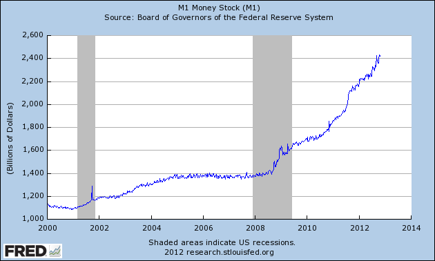
Roughly, the nation’s money supply at any given moment is the total amount of liquid assets —that is, assets that can easily be used to pay for purchases when you go shopping—that are held by private citizens at that moment. A popular measure of money supply is M1. It consists of all currency in private hands and all the money in people’s checking accounts. You may think of M1 as the maximum amount of money that people would be able to spend if they all went shopping this minute. See Figure 5.4 for recent trends in M1 for the United States. For instance, on October 22, 2012, M1 was an estimated $2,417.2 billion, of which currency in private hands was $1,079.2 billion, total checkable deposits was $1,334.0 billion, and travelers checks outstanding was $3.9 billion.

Figure 5.4: One measure of money supply is M1. Here we see recent US data on M1. Note that the Federal Reserve’s actions tend to sharply boost money supply in recessions. We will see why in later chapters. Source: https://fred.stlouisfed.org/series/M1SL.

As we saw in Section 1.4.2, I will denote money supply by the symbol $M$.

5.8.2 What Are the Factors that Affect Money Supply?

A nation’s money supply is controlled by its central bank.¹¹ Recall that M1, the simplest measure of $M$, is basically equal to the currency held by the public and the value of all checkable bank accounts. The central bank can use its power to affect both these components of M1. The central bank is the only institution that can print (or mint) currency. Therefore, the “currency held by the public” can increase only if the central bank buys something from John or Jane Q. Public and pays for it with newly printed cash.

For instance, if Jane decides to sell some of the government bonds that she owns, she may end up selling her bonds to the central bank in return for a bunch of newly printed currency notes. This would imply an increase in the currency held by the public and, therefore, in M1. Or, it could be that John has some yen that he wishes to sell in return for dollars. John could end up selling his yen to the U.S. central bank, which is known as the Federal Reserve or, simply, The Fed. Again, he would be paid in crisp newly printed dollar bills, the currency held by the public would increase, as would M1.

Of course, the central bank could just as easily decide to sell some of its financial assets. In that case, the above process would work in reverse and M1 would decrease. If the Fed decides to sell some of the government bonds it owns, the buyer could be one John Q. Public. In this case, John would hand over some not-so-crisp dollar bills from his wallet to the Fed as payment for the bonds he had just purchased. Consequently, the currency held by the public would decrease, as would M1.

Apart from controlling the currency held by the public in the manner just outlined, a central bank indirectly controls “the value of all checkable bank accounts”, which is the other component of M1. This is because a central bank typically has the power to regulate the lending behavior of banks. If I walk into a bank and deposit a hundred dollars into my account, the bank manager would lend $X$ dollars out of the money I had deposited to someone who wants a loan. That man may use the $X$ dollars he had borrowed to buy a shirt, in which case those $X$ dollars would end up in the shirt seller’s checkable bank account. Therefore, M1 would increase by $X$ dollars. In other words, the lending of depositors’ money by banks can affect M1.

And that’s where the central bank can use its regulatory power to control the value of all checkable bank accounts and, thereby, M1. The central bank can set limits on how much of my hundred-dollar deposit my bank could lend. By adjusting the limit the central bank can encourage the manager of my bank to lend more or less than $X$ dollars to the guy who wanted a loan. Thereby, the central bank can (indirectly) control the rate at which bank lending expands M1.

In some cases, central banks give up control over the money supply in order to exert control over some other economic variable that they consider important to control. You will see in Chapter 8 that in what are called fixed exchange rate systems, the central bank can fix the value of a currency by credibly promising to buy and/or sell that currency at the target rate of exchange. For example, if the central bank of Thailand wishes to fix the exchange value of the Thai baht at 25 bahts per US dollar, it can do so by announcing that it is ready to buy and/or sell US dollars at the rate of 25 bahts per dollar. After that announcement, the market price of a dollar could not be, say, 27 baht because nobody would buy a dollar at that price when Thailand’s central bank is willing to sell dollars for less. Similarly, the price of a dollar could not be 23 baht because nobody would sell at that price given that they could instead sell dollars to the Thai central bank for a higher price. In short, once Thailand’s central bank makes a credible announcement that it will exchange one dollar for 25 baht, the market exchange rate of a dollar will quickly become 25 baht.

However, the Thai central bank’s efforts to control the exchange rate of the baht must come at the expense of its total loss of control over Thailand’s M1. If people show up with dollars and ask for baht, the central bank would have to print some additional currency. So, currency held by the public would increase, as would M1. If some Thai citizens hand over their baht and ask for dollars, the central bank would have to dig into its dollar reserves to keep its promise. The baht held by the thai public would decrease (because they have exhanged some of their baht for dollars), as would M1. In this way, the central bank would gain some control over the exchange rate, but by giving up control over M1. M1 would now fluctuate not according to the wishes of the Thai central bank but in tune with economic conditions in Thailand or, indeed, the world at large.

5.8.3 What Is the Money Demand?

The nation’s money demand at a specified point in time is the total amount of liquid assets—that is, currency plus checkable bank accounts—that its residents would like to hold at that point in time.

5.8.4 What Are the Factors that Affect the Demand for Money?

The behavior of the demand for money is assumed to be described by the equation \[ \text{Money Demand}=L(R)\cdot P\cdot Y. \]

In other words, the demand for money is assumed to be a multiple $L$ of nominal income ($P\cdot Y$; see Equation 2.12 of Section 2.6.1). Moreover, the multiple $L$ itself depends on the nominal interest rate ($R$).

5.8.4.1 What Are Nominal Interest Rates?

The nominal interest rate, denoted by $R$ for the domestic country and $R^*$ for the foreign country, is the fraction of each currency unit borrowed (dollar, yen, etc.) that will have to be paid as interest.¹² If the bank charges you 15% interest on a loan, then the nominal interest rate is $R=0.15$ because that is the fraction of each dollar borrowed that you will have to pay as interest.

5.8.4.2 Again, What Are the Factors that Affect the Demand for Money?

As is clear from the equation above, the demand for money is assumed to vary directly with $P$ and $Y$. This makes sense. If, other things being unchanged, the average price level ($P$) goes up, wouldn’t you wish to keep a larger part of your wealth as cash in your wallet? Of course, you would. And if GDP ($Y$) increases, wouldn’t people carry more cash in their wallets? Of course, they would. A higher real GDP implies that more goods and services are being produced and then bought and sold. All this extra buying and selling will require people to carry more cash with them on a regular basis.

And, as for the effect of $R$ on money demand, if the nominal interest rate increases, wouldn’t you wish to keep less of your wealth in cash? Yes, you would. Keep in mind that liquid assets, such as cash and checking account deposits, are convenient when you need to go shopping, but earn little or no interest. The nominal interest rate $R$ is the interest rate on non-liquid assets , such as bonds. So, a higher nominal interest rate increases the attractiveness of non-liquid assets and thereby reduces the desirability of liquid assets. Therefore, $R$ and $L$—and, therefore, $R$ and money demand—are inversely related.¹³

Other factors matter too. For example, in an economic crisis, when people are unsure that borrowers will be able to repay their loans, they may keep more of their wealth in the form of cold hard cash instead of lending it to others. On the other hand, when people are wealthier, they would very likely carry more cash.¹⁴

5.8.5 Summary: What Is the Money Market Equilibrium Condition?

The necessary equality of the supply and demand for money gives us what is usually called the money market equilibrium condition :

\[ \fbox{$\displaystyle M=L(R)\cdot P\cdot Y.$} \tag{5.9}\]

5.9 What Is the Equilibrium Condition for the Foreign Exchange Market?

Foreign exchange markets are said to be in equilibrium if, for any two currencies $A$ and $B$, the amount of Currency $A$ supplied—by those who wish to sell Currency $A$ in exchange for Currency $B$—is equal to the amount of Currency $A$ demanded—by those who wish to sell Currency $B$ in exchange for Currency $A$. For this to be true, uncovered interest arbitrage must not be possible.

People may wish to exchange currency $A$ for currency $B$ for many reasons. They may be tourists who have currency $A$ but wish to travel in regions where currency $B$ is accepted. They may be people who have currency $A$ but wish to buy goods, services, or assets from people who accept only currency $B$. However, I will focus on one particular reason why people trade currencies: it involves speculation (or, less politely, financial gambling) and is called uncovered interest arbitrage. The foreign currency markets are in equilibrium when the demand and supply from these speculators are perfectly matched.

5.9.1 What Is Uncovered Interest Arbitrage?

Opportunities for uncovered interest arbitrage are said to exist if one can expect to profit by borrowing money in country $A$ and lending it to borrowers in country $B$, or vice versa.¹⁵ If this is possible, then there would be no equilibrium in the foreign exchange market. Profit seekers would be constantly borrowing money in country $A$ and then changing it into the currency of country $B$ for the purpose of lending it to borrowers in that country. There would be literally no limit to the amount of country $A$’s currency supplied by these people and—for the same reason—no limit to the amount of country $B$’s currency demanded by these people. As a result, the supply of country $A$’s currency would necessarily exceed the demand for it. Such a situation would not represent equilibrium.

Therefore, for equilibrium in foreign exchange markets, there must not exist any opportunities for uncovered interest arbitrage. Put another way, the uncovered interest parity condition must be satisfied.

5.9.2 What Is the Uncovered Interest Parity Condition?

The uncovered interest parity condition (UIP, for short) is that \[ R=R^*+\frac{E^e_f-E}{E} \tag{5.10}\] must be satisfied.

As we saw in Section 5.8.4.1 above, $R$ is the nominal interest rate in the home country, whereas $R^*$ is the nominal interest rate in the foreign country. As we saw in Section 4.1, $E$ is the current value of the foreign currency in units of the domestic currency. And, as we saw in Section 4.4.1, $E_f$ is the future value of the foreign currency, and $E_f^e$ is the current expectation of the future value of the foreign currency.¹⁶

Note that $E^e_f-E$ is the expected increase in the exchange value of the foreign currency. It then follows—along the lines of Equation 2.3 in Section 2.3.1 — that \[ \begin{eqnarray} E^e_g&\equiv&\frac{E^e_f-E}{E}\nonumber \\ &\equiv&\frac{E^e_f}{E}-1 \end{eqnarray} \tag{5.11}\] is the expected proportional rate of increase of the exchange value of the foreign currency. The uncovered interest parity equation above can therefore be written compactly as \[ R=R^*+E_g^e. \tag{5.12}\]

The second term on the right-hand side, $E_g^e$, is often called the expected rate of appreciation of the foreign currency . When the exchange value of a currency increases (respectively, decreases), the currency is said to have appreciated (respectively, depreciated) .¹⁷

With the definitions of the variables in Equation 5.10 out of the way, we can now try to understand why that equation makes sense.

5.9.2.1 Why Is Uncovered Interest Parity Necessary for Equilibrium?

To see the meaning of Equation 5.10 above, consider the prospect of borrowing US dollars from someone in America today, turning it into euros in the foreign exchange market, lending it to someone in Europe for a year, turning the euros received a year later (as principal and interest on the loan that was made) back into dollars, paying off the dollars that had been borrowed a year earlier, and keeping any profits or losses that remain.

The downside of this plan is that you would have to pay interest $R$ on the money you borrowed in America. This is on the left-hand side of the UIP equation; i.e., Equation 5.10.

But there is an upside too. You will get interest $R^*$ from your borrowers in Europe.

And that is not all. Remember that the plan requires you to change your borrowed dollars into euros today and then change your euros back into dollars a year later. So, you would make some money if the nominal value of the euro, $E$, grows during the year. For example, if $E = 2$ today, you would pay $2.00 for every euro you buy today. And if $E_f^e = 4$ a year later, you would be able to turn each euro you have into $4.00. So, if $E$ grows from $E = 2$ at the beginning of the year to $E^e_f = 4$ at the year’s end, you could turn $2.00 into $4.00 over that year. In general, $E^e_g\equiv(E^e_f-E)/E$ represents your expected gains from changing dollars into euros and back into dollars a year later.

Therefore, the right-hand side of the UIP equation above—i.e., $R^* + E^e_g$—represents your total gains from this convoluted scheme of borrowing dollars, changing it into euros, earning interest on those euros for a year, and finally changing the euros back into dollars and bringing the money home.

Had the left-hand side ($R$) been smaller than the right-hand side ($R^* + E^e_g$), opportunities for uncovered interest arbitrage would have existed. That is, you (and everybody else in the world) would have profited from borrowing in America and lending that money in Europe. But that would have violated the equilibrium condition for the foreign exchange markets.

In the same way, it can be shown that had the left-hand side been greater than the right-hand side, opportunities for uncovered interest arbitrage would once again have existed. Only, this time you would expect to gain by borrowing in Europe and lending in America.

So, for equilibrium in the foreign exchange market, the two sides of Equation 5.10 would have to be equal. That is, for equilibrium in the foreign exchange market, the uncovered interest parity condition must be satisfied. This can be expressed either by Equation 5.10 or, equivalently, by \[ \fbox{$\displaystyle R=R^*+\frac{E^e_f}{E}-1.$} \tag{5.13}\]

5.9.2.2 Perfect Capital Mobility

My discussion of the uncovered interest parity condition in Section 5.9.2.1 has implicitly assumed perfect capital mobility in foreign exchange markets. This requires that:

All individuals have the same expectations, and
When considering which assets to buy and which assets to sell, people only look at the long-run average returns of the various available assets.¹⁸

The first requirement was discussed in Section 5.9.2 on $E_f^e$.

The second requirement of perfect capital mobility is that the long-run average return of an asset is all that we care about when judging the attractiveness of an asset. This idea is implicit in the discussion of uncovered interest parity in Section 5.9.2.1. If you borrow money in America and lend it in Europe, the benefits of all this wheeling and dealing are measured by $R^*+[(E^e_f-E)/E]$. This is just the long-run average return that you would expect to receive. The UIP equation, Equation 5.10, therefore, reflects what equilibrium in foreign exchange markets ought to look like if these long-run average returns are all that matter to people.

Perfect capital mobility, therefore, implies that the UIP equation must be satisfied for the foreign exchange market to be in equilibrium.

We need to remember, however, that although I have assumed perfect capital mobility, I did so just for simplicity. In the real world, perfect capital mobility is unlikely to be true. First of all, different people cannot be expected to have the same expectations. Secondly, in judging the attractiveness of an asset, people are likely to look not only at the asset’s long-run average return but also at the volatility (or variability, or dispersion, or riskiness) of the asset’s return. Consider asset $A$, which gives a steady 5% return, and another asset, asset $B$, which yields a 0% return half the time and a 10% return half the time, for a long-run average return of 5%. Assets $A$ and $B$ both have the same long-run average return of 5%. And yet, most people will not regard assets $A$ and $B$ to be equally attractive; most people will regard asset $A$ to be superior because it is less risky.

In my justification of uncovered interest parity in Section 5.9.2.1, I focused on the long-run average returns and ignored the riskiness of assets. For example, I assumed that people consider $(E^e_f-E)/E$, the expected appreciation of the foreign currency, but ignore the fact that even if people have an expectation about how much that currency may appreciate, they will also be aware that that expectation is just that, an expectation.

Therefore, one needs to keep in mind the limitations inherent in defining equilibrium in foreign exchange markets by Equation 5.10.

5.10 Summary: The Basic Equations

To sum up, the theory of international macroeconomics that I am discussing here—which, incidentally, is called the Mundell-Fleming theory after the names of its authors—relies on three basic equations:

The goods market equilibrium equation that must be satisfied if the demand for domestically produced goods is to be equal to the supply of such goods. See Equation 5.1, and Equation 5.8 for equivalent versions of this equation.
The money market equilibrium equation that must be satisfied if the demand for money is to be equal to the supply of money. See Equation 5.9.
The foreign exchange market equilibrium equation that must be satisfied if the demand for foreign currencies is to be equal to the supply of foreign currencies. See Equation 5.10 and Equation 5.13 for equivalent versions of this equation.

To be precise, in Equation 2.8, $Y$ denotes gross national domestic income, which is slightly different from gross domestic product, and $CA$ denotes the current account balance which is slightly different from $NX$ or net exports. However, these small differences—see Section 2.5.1.2 and Section 2.5.1.3 — are not the main issue here. The main distinction between Equation 5.1 on the one hand and the national income identity—that is, Equation 2.5 or Equation 2.8 — on the other is that Equation 5.1 has a theoretical justification, whereas Equation 2.5 and Equation 2.8 are true by virtue of how the variables in them are defined by statisticians. The theory that says that Equation 5.1 is true may be false. But the national income identity is necessarily true by virtue of the definitions of the variables in it.↩︎
Readers may recall a parallel discussion of the national income identity in Section 2.5.↩︎
Note that $Y$ is defined as the supply of goods planned by domestic producers. If the producers’ desires are fulfilled, $Y$ would also be the actual sales of domestic producers. Therefore, $Y$ would also be the total income of households because the total sales of final goods must also be equal to total earnings. After all, if ten trillion dollars worth of “Made in USA” goods were produced and sold last year, how did the ten trillion dollars that buyers paid for those goods end up? As the incomes of all the people involved in their production, of course.↩︎
Note that $0<\hbox{MPC},\hbox{MPS}<1$ and that $\hbox{MPC}+\hbox{MPS}=1$, by definition.↩︎
For a full discussion, see pages 163-5 of Macroeconomics: A Modern Approach by Robert J. Barro, Thomson South-Western, Mason, OH, 2008.↩︎
The government could take out a new loan to repay an old loan. But there are limits to how far this could be continued. Lenders may eventually balk.↩︎
Indeed, in a later chapter I will assume that real investment spending, $I$, is inversely related to the real interest rate, $r$.↩︎
See chapter 17 of Macroeconomics, sixth edition, by N. Gregory Mankiw, Worth Publishers, New York, NY, 2007, ISBN:978–0–7167–6213–3, for more on the theory of business investment.↩︎
I should not, however, give the impression that factors that influence the level of government spending are not discussed in economic research. See Mueller (2003), Persson and Tabellini (2002), and Drazen (2002).↩︎
See Section 10.4 of Chapter 10. ↩︎
See Section 3.3.↩︎
Recall from Section 4.2.1 that the variables that describe a foreign country have an asterisk (*) attached as a superscript.↩︎
The factor $L$ is the reciprocal of what is called the velocity of money or the income velocity of money, $V$. That is, $L=1/V$. The velocity is defined as the average number of times per period that a unit of currency is used in the purchase of a final good or service. For example, if the average dollar bill changes hands 10 times per month, then $V=10$.↩︎
During the recession of 2008–09, many people who had borrowed money to buy homes, defaulted on their loans when home prices, which they had thought would keep rising, fell instead. This shocking rise in loan defaults made lenders afraid to lend money. The sudden decline in the availability of loans made it hard for businesses to borrow money to expand. The sales of new homes and cars fell sharply because consumer loans dried up. All this led to sharp declines in real GDP and sharp rises in unemployment in the US. These troubles in the US had serious negative effects on other countries as well.↩︎
In the business press, uncovered interest arbitrage is also referred to as the “carry trade.” See, for example, “Why the ‘Carry Trade’ Is Back,” by Neil Shah, The Wall Street Journal, August 18, 2009, https://www.wsj.com/articles/SB125053694840237795. ↩︎
Note that, I have quietly assumed that everybody has the same expectation for the future value of the foreign currency; no differences of opinion are allowed. Also, you may recall that $E_f^e$ was introduced earlier in Section 4.4.↩︎
Similarly, $100\times[(E^e_f-E)/E]$ is the expected percentage rate of increase of the exchange value of the foreign currency. Note that when $E^e_f<E$, we have a negative expected increase, which is the same as a decrease.↩︎
The long-run average return of an asset is also called the mathematical expectation of the returns of the asset.↩︎