11 Short-Run Predictions: Fixed Exchange Rates

In the last two chapters, we have seen how a country is affected in the long run by permanent changes in exogenous variables. For example, we saw in Chapter 9 that a permanent cut in government spending ($G\downarrow$) leads to an increase in a country’s net exports ($NX\uparrow$) in the long run. And in Chapter 10 we saw that in the long run a permanent increase in the foreign inflation rate ($\pi^*$) will raise the domestic inflation rate ($\pi$) under fixed exchange rates but not under flexible exchange rates.¹

The questions that we wrestle with in this and the next two chapters are not about the long run. Specifically, our questions will now follow this general format: If there is an increase in [some exogenous variable], what will happen in the short run to [some endogenous variable]? If a country is hit by a recession and lots of people begin to lose their jobs, what could turn things around in a relatively short amount of time? Would a temporary tax cut have the desired effect? The relevance of such questions is obvious.

This chapter considers an economy that has a fixed exchange rate system.² The next two chapters will consider flexible exchange rates. Although flexible exchange rate systems are far more widespread than fixed exchange rate systems, I chose to discuss fixed exchange rates first mainly because the analysis is somewhat simpler.

11.1 The short run needs a different approach

But first, why do we need separate chapters for long-run analysis and short-run analysis? Why can’t we make do with the last two chapters? Why wouldn’t the long-run analysis of the last two chapters be applicable in the short run as well?

11.1.1 Recessions and Booms

To see why, recall from Section 7.2 that long-run analysis assumes full employment. That is, an economy’s real gross domestic product ($Y$) is assumed to be equal to its potential real gross domestic product ($Y^p$). In other words, recessions and booms are ruled out by assumption. This short-cut is fine for long-run analysis, but not for short-run analysis.

Sudden and sharp declines in $Y$ do happen. Therefore, such recessions need to be explained. A theory that assumes $Y=Y^p$ can “explain” a sharp decline in $Y$ by arguing that there must have been a sharp decline in $Y^p$. But such an explanation is unpersuasive. After all, as we saw in Section 7.2.1, the factors that determine a country’s potential GDP—the quantity and quality of productive resources, the level of technology, and the nature of the country’s institutions—typically do not go up and down like a yoyo. Therefore, for short-run analysis, the only way to reconcile a stable $Y^p$ with a volatile $Y$ is by rejecting the $Y=Y^p$ assumption and admitting that recessions ($Y<Y^p$) and booms ($Y>Y^p$) may happen.

11.1.2 Price Rigidity

A related question is this: What might make $Y$ less than $Y^p$? If an economy is capable of producing $14 trillion worth of goods and services per year under normal circumstances, why would it not produce that amount? Why would it produce less? Or more? The key reason is that prices tend to be sticky (or ‘rigid’ or ‘inflexible’) in the short run.

In the long run, changes in the price level ($P$) tend to yank $Y$ towards $Y^p$ whenever the two diverge. In recessions ($Y<Y^p$), unemployment rises. The availability of many unemployed workers seeking jobs tends to make labor cheaper. This induces businesses to hire additional workers and boost production. To sell the additional output, firms must reduce prices, and indeed they can afford to do so because the wages they pay their workers have fallen. So, a recovery occurs and $Y$ again becomes equal to $Y^p$ thanks to the flexibility of wages and prices. This ability of the price level to respond flexibly to a recession and restore full employment is what makes the $Y=Y^p$ assumption reasonable in long-run analysis.

Unfortunately, this smooth self-adjusting process tends not to work in the short run. In the short run, wages may not fall in a recession—the presence of many unemployed job seekers notwithstanding—because of contracts that were agreed upon among businesses and workers or because of several other reasons. Wages are sticky in the short run. And, the stickiness of wages typically means sticky prices as well. Moreover, prices may be sticky for reasons unrelated to the stickiness of wages. And this price stickiness could make it difficult for businesses to hire more workers during a recession because the additional output produced by the newly hired workers will not sell if prices cannot be reduced.

11.1.3 Expectations

Another distinction between long-run analysis and short-run analysis has to do with expectations. As we saw in Section 7.3, short-run analysis assumes that $E_f^e$, which is what the value of the foreign currency at a future date is currently expected to be, is equal to $E_{fLR}$, which is the long-run equilibrium value of $E_f$. Moreover, $E_{fLR}$ is assumed to be exogenous. Long-run analysis, on the other hand, assumes perfect foresight: $E_f^e=E_f$. This is equivalent to the $E_f^e=E_{fLR}$ assumption of short-run analysis except that $E_{fLR}$ is endogenous in long-run analysis.

The distinction is hard to explain, but let me try. For both long-run analysis and short-run analysis we assume $E_f^e=E_{fLR}$. That is, we assume that people’s expectations about $E_f$ will coincide with its actual long-run equilibrium value. In long-run analysis, as we saw in Section 10.8.6, $E_f$ is an endogenous and unknown variable—like $E$, $R$, $P$, $\pi$, etc.—whose equilibrium value is determined by the theory itself; that is why Table 10.1 has an entire column listing how the various exogenous variables affect the long-run equilibrium value of $E_f$. Short-run analysis, on the other hand, is unable to determine the value of $E_{fLR}$. It treats $E_{fLR}$ as a mysterious, exogenous variable that dances to its own tune. It has to seek the assistance of long-run analysis to understand what makes $E_{fLR}$ increase or decrease.

The distinction between the long-run and short-run assumptions about expectations is key to understanding why the short-run effects of a temporary change in an exogenous variable are different from the short-run effects of a permanent change in that same exogenous variable. A temporary change in an exogenous variable—for example, a temporary cut in taxes ($T\downarrow$)—cannot be expected to affect the future. Therefore, it makes sense to assume that people’s expectations about the future ($E_f^e$) will be unaffected. As a result, the short-run analysis of a temporary tax cut can proceed on the assumption that $E_f^e$ has not changed. The short-run analysis of a permanent tax cut is a more complex matter. Table 10.1, which summarizes the long-run analysis of a flexible exchange rate system, says that a permanent tax cut will reduce $E_{fLR}$. Knowing this, the people will rationally revise $E_f^e$ downward as soon as the permanent tax cut is announced. Therefore, the short-run effect of a permanent tax cut is the combined effect of a temporary tax cutand a decrease in $E_f^e$.

We will discuss this issue further in the next two chapters.

11.2 Short-Run Equilibrium in the Goods Market

We are now ready to do what we did in Chapter 9 and Chapter 10, but under the short-run assumptions that both $P$ and $E_f^e$ are exogenous. Unfortunately, short-run analysis is not as straightforward as long-run analysis. The arguments will have to be built up brick-by-brick and a full view of the theory will not be visible for quite a while. You will have to be patient.

The foundation of the theory will once again consist of the equations for equilibrium in the goods, money, and foreign currency markets that we saw in Chapter 5. So, it might be a good idea for you to review Equation 5.8, Equation 5.9, and Equation 5.13.

11.2.1 The Aggregate Expenditure Curve

Recall from Section 5.1 that equilibrium in the goods market requires that the demand for domestically produced goods be equal to the output of such goods, as in Equation 5.8. This crucial equation is reproduced below, with Equation 4.1 or $q=E\cdot P^*/P$ substituted for $q$: \[ \fbox{$\displaystyle Y=C(Y-T)+I+G+NX\left(\frac{E\cdot P^*}{P},Y-T\right).$} \tag{11.1}\]

Note that $Y$ is the only endogenous variable in the above equation. As we saw in Section 7.1 that $T$, $I$, $G$, and $P^*$ are always exogenous in these lectures. Moreover, as we saw above, $P$ is exogenous in short-run analysis. And, finally, $E$ is exogenous because we are considering fixed exchange rates in this chapter. That leaves $Y$ as the only endogenous variable in Equation 11.1. This implies that an analysis of this equation will tell us all that can be said about the short-run behavior of $Y$ under fixed exchange rates.³

The analysis of Equation 11.1 will now proceed, not algebraically but graphically. (Indeed, you will see that a lot of short-run analysis is graphical.)

As was mentioned in the first paragraph of this section, the right-hand side of Equation 11.1 represents the total expenditure on domestically produced goods. This is usually referred to as aggregate expenditure or $AE$. The goods market equilibrium condition can then be stated simply as $Y=AE$. $C$, $I$, $G$, and $NX$ are called the *components of aggregate expenditure.⁴

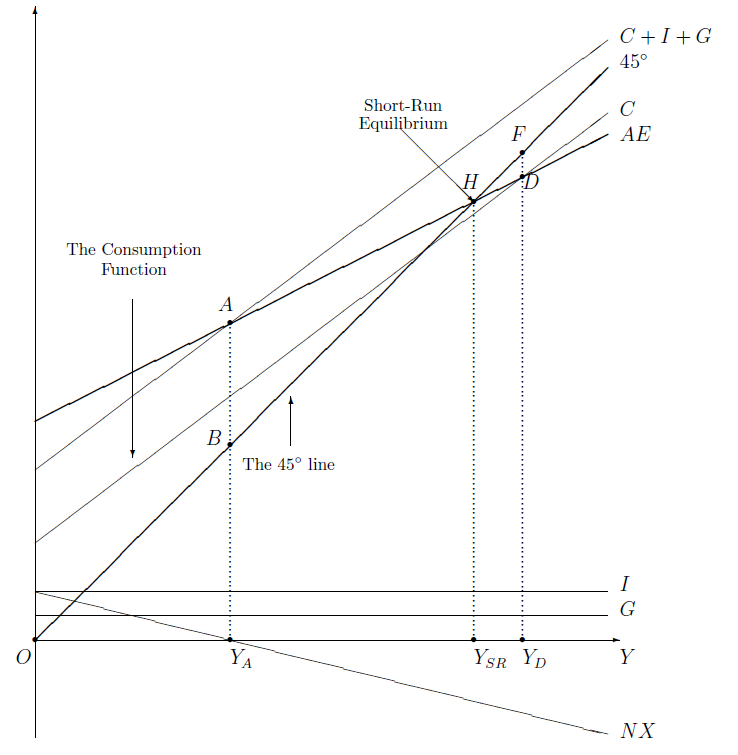
We saw in Section 5.3 that a country’s consumption spending ($C$) is represented by the consumption function $C=C(Y-T)$. We assume that $C$ is directly related to income ($Y$) and inversely related to taxes ($T$). Figure 5.1 showed the consumption function graphically as a rising consumption curve. Moreover, Figure 5.1 also shows that the consumption curve shifts downward when taxes increase. The consumption curve of Figure 5.1 makes a return appearance in figure Figure 11.1 in this chapter.

As we saw in Section 5.4 and Section 5.5, business investment ($I$) and government spending ($G$) are assumed to be exogenous constants; in particular, they do not go up or down when $Y$ increases or decreases. In figure Figure 11.1 they are therefore represented by horizontal lines.

If we stack the $C$, $I$, and $G$ curves one on top of the other, we get the $C+I+G$ curve in figure Figure 11.1. $C+I+G$ is commonly referred to as gross domestic purchases, the total purchases of domestic households, firms, and government.

We saw in Section 5.6.3 that a country’s net exports are given by $NX=NX(q,Y-T)$ and that net exports are directly related to the real exchange rate ($q$) and to $T$, and inversely related to $Y$. Figure Figure 5.2 showed this graphically. Its right panel, in particular, shows a net exports curve that slopes downward as $Y$ increases and shifts downward when either $q$ or $T$ falls. This net exports curve makes a return appearance in figure Figure 11.1 here.

If we stack the $C$, $I$, $G$, and $NX$ curves vertically, we get the aggregate expenditure ($AE=C+I+G+NX$) curve in figure Figure 11.1. At any particular value of real GDP ($Y$), the height of the $AE$ curve shows the total demand for domestically produced goods.

11.2.2 Slope of the Curve

Note that the $AE$ curve is upward sloping. Would it be a mistake to draw it as a downward-sloping curve instead? Recall that the $I$ and $G$ curves are horizontal, the $C$ curve is upward sloping, and the $NX$ curve is downward sloping. When these curves are stacked vertically to construct the $AE$ curve, couldn’t the result be a downward-sloping curve?

Well, no. A quick look at Section 5.6.2 will settle the issue. When income ($Y$) increases, so does consumption ($C$). Only a part of that additional consumption is imported. That is, imports increase, but by less than the magnitude of the increase in consumption. As exports are unaffected by $Y$, net exports ($NX$) will decrease, but again by less than the magnitude of the increase in $C$. Therefore, $AE=C+I+G+NX$ will increase when $Y$ increases, which means that the $AE$ curve in figure Figure 11.1 has been quite properly shown to be upward sloping.

Note that $NX$ can be positive or zero or negative. At $Y=Y_A$ in figure Figure 11.1, $NX=0$, which is why the gross domestic purchases ($C+I+G$) curve and the aggregate expenditure ($AE=C+I+G+NX$) curve have the same height (that is, they intersect) at $Y=Y_A$. At lower incomes ($Y<Y_A$), $NX>0$ and, therefore, $AE$ exceeds $C+I+G$. At higher incomes ($Y>Y_A$), $NX<0$ and, therefore, $AE$ is less than $C+I+G$.

11.2.3 The 45 Line

Figure Figure 11.1 also includes a 45$^{\circ}$ line through the origin. To see the utility of this seemingly useless line, note that at any value of $Y$, the height of the 45$^{\circ}$ line is equal to the value of $Y$. For instance, at $Y=Y_A$, the height up to point $B$ on the 45$^{\circ}$ line is equal to $Y_A$, whereas the height up to point $A$ on the $AE$ curve exceeds $Y_A$. As the height of the $AE$ curve denotes the magnitude of $AE=C+I+G+NX$, it follows that at $Y=Y_A$, $Y<AE$, which violates Equation 11.1, the equilibrium condition for the goods market. So, simply by noting that the $AE$ curve is higher than the 45$^{\circ}$ line at $Y=Y_A$, one can conclude that it would be unwise to predict that $Y=Y_A$ in short-run equilibrium.

Figure 11.1: Here we see how the short-run equilibrium value of $Y$ can be graphically determined if the aggregate expenditure curve ($AE$) is known. The $AE$ curve is constructed by the vertical summation of the consumption ($C$), investment ($I$), government spending ($G$), and net exports ($NX$) curves. The goods market is in equilibrium when $Y=AE$—that is, when the $AE$ curve intersects the 45$^{\circ}$ line.

11.2.4 The Keynesian Cross

Now that we have ruled out $Y_A$, could the short-run equilibrium value of $Y$ be $Y_D$ instead? At $Y=Y_D$, a comparison of points $D$ and $F$ shows that the height of the $AE$ curve is less than the height of the 45$^{\circ}$ line. Therefore, $Y>AE$ at $Y=Y_D$. So, $Y_D$ can’t be the short-run equilibrium GDP either.

So far, we have tried twice to spot the equilibrium value of $Y$ and have failed miserably. At $Y_A$, the $AE$ curve was higher than the 45$^{\circ}$ line. At $Y_D$, the $AE$ curve was lower than the 45$^{\circ}$ line. So, it makes sense to try point $H$ where the two curves cross. At $Y=Y_{SR}$, the heights of the two curves are same, implying $Y=AE$. Therefore, the short-run equilibrium value of real GDP must be $Y=Y_{SR}$.

That’s it, we’ve finally got it! We have established that if a country’s $AE$ curve is known, its short-run equilibrium GDP is the value of $Y$ at which the $AE$ curve crosses the 45$^{\circ}$ line.

As you will soon see, this graphical trick will be very useful in predicting how GDP is affected by changes in various exogenous variables.

Figure 11.2: An upward shift of the aggregate expenditure curve leads to an increase in GDP in the short run. Such an upward shift of the $AE$ curve could be caused by an increase in $G$ or $I$ or $E$ or $P^*$, or by a decrease in $T$ or $P$, or by some combination of these changes. Therefore, in the short run and under fixed exchange rates, $Y$ is directly affected by $G$, $I$, $E$, and $P^*$; inversely affected by $T$ and $P$, and unaffected by all other exogenous variables.

11.2.5 Gross Domestic Product: How the $AE$ curve can shift

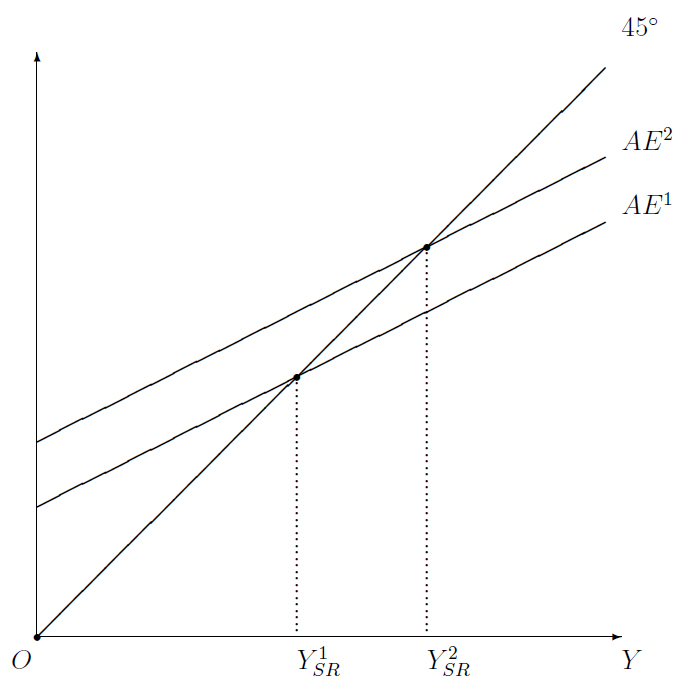
In figure Figure 11.2, there are two aggregate expenditure curves, $AE^1$ and $AE^2$, as well as the 45$^{\circ}$ line that first appeared in figure Figure 11.1. Given that the short-run equilibrium level of income is that at which the $AE$ curve crosses the 45$^{\circ}$ line, it follows that equilibrium income must be $Y_{SR}^1$ when aggregate expenditure is $AE^1$ and $Y_{SR}^2$ when aggregate expenditure is $AE^2$. In other words, the higher the $AE$ curve, the higher the short-run equilibrium income.

Therefore, if we knew what makes the aggregate expenditure curve rise, we would know what makes income increase.

Luckily, it is straightforward to figure out what makes the $AE$ curve rise (or fall). Recall from Section 11.2.1 that the $AE$ curve is the vertical sum of the $C$, $I$, $G$, and $NX$ curves. Therefore, anything that causes any of these curves to shift upwards will also shift the $AE$ curve upwards.

We saw in Section 5.3 and figure Figure 5.1 that a decrease in taxes ($T\downarrow$) shifts the $C$ curve up. An increase in households’ wealth—possibly fueled by a rise in share prices or home prices—would have the same effect, as would a general surge in optimism. Therefore, any combination of these factors would shift the $AE$ curve upwards as well.

A surge in optimism among entrepreneurs will cause business investment to increase. This would raise the $I$ curve and, therefore, the $AE$ curve.

A shift in government policy—brought about, say, by the election of a new president—could boost government spending. This would raise the $G$ curve and, consequently, the $AE$ curve.

As was pointed out in Figure 5.2, an increase in either taxes ($T\uparrow$) or the real exchange rate ($q\uparrow$) shifts the net exports curve upwards. Of course, we know from Equation 4.1 that $q=E\cdot P^*/P$. Therefore, we can say that the $NX$ and $AE$ curves would shift upwards if $E$ increases or $P^*$ increases or $P$ decreases. In all these cases, the $NX$ curve rises and, therefore, so does the $AE$ curve.⁵

There is a slight problem, however, with the effect of taxes. A tax cut ($T\downarrow$) raises the $C$ curve and lowers the $NX$ curve, simultaneously. What’s the overall effect on these conflicting effects on the $AE$ curve? As this issue was addressed indirectly in Section 11.2.2, I don’t want to rehash the argument here. Long story short, when taxes fall, consumption increases and so do imports, but by a smaller amount. As a result, the $C$ curve shifts up and the $NX=\hbox{exports}-\hbox{imports}$ shifts down, but the increase in $C$ exceeds the decrease in $NX$. Therefore, the $AE$ curve shifts up.

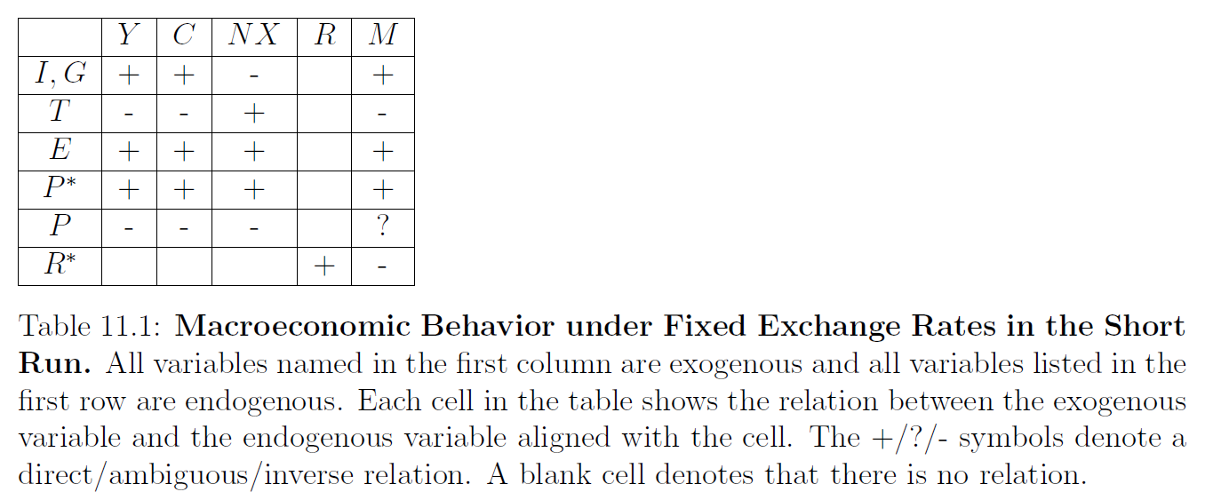
To summarize, in an economy that has a fixed exchange rate system, the aggregate expenditure curve shifts upwards—and, therefore, short-run equilibrium income ($Y$) rises—if there is a ceteris paribus decrease in $T$ or $P$, or there is a ceteris paribus increase in $I$ or $G$ or $E$ or $P^*$, or there is some combination of those changes. Changes in other exogenous variables will have no effect. This is shown in the $Y$-column of Table 11.1.

11.2.6 Consumption

What can we say about the short-run behavior of consumption spending under fixed exchange rates? For example, how will $C$ react if $T$ increases? Recall that $C=C(Y-T)$. We have just seen that $Y$ decreases when $T$ increases. This decrease in $Y$ coupled with the increase in $T$ implies that disposable income ($Y-T$) will decrease. Therefore, $C$ must decrease.

Changes in the other exogenous variables—$I$, $G$, $P^*$, $E$, and $P$—cannot affect $T$, which is exogenous. Therefore, their effects on $C=C(Y-T)$ will be the same as their effects on $Y$. That is why the $C$ and $Y$ columns of Table 11.1 are the same for these five exogenous variables.⁶

To summarize, in an economy that has a fixed exchange rate system, in the short-run equilibrium, $C$ is directly affected by $I$, $G$, $P^*$, and $E$, inversely affected by $T$ and $P$, and unaffected by all other exogenous variables. These ceteris paribus effects are shown in the $C$-column of Table 11.1.

11.2.7 Net Exports

To analyze the behavior of net exports, I will make use of the behavioral expression $NX=NX(E\cdot P^*/P,Y-T)$ and the goods market equilibrium condition, which yields $NX=Y-C(Y-T)-I-G$.⁷

First, consider an increase in $I$ or an increase in $G$ or a decrease in $T$. The $Y$-column of Table 11.1 assures us that $Y$ will increase. Therefore, disposable income ($Y-T$) will increase too. Moreover, $E\cdot P^*/P$ will be unaffected as $E$, $P^*$, and $P$ are all exogenous and, therefore, cannot be affected by changes in other exogenous variables. Therefore, $NX=NX(E\cdot P^*/P,Y-T)$ must decrease, as net exports fall when rising disposable income leads to surging imports—see Section 5.6.

Second, check from Section 11.2.5 of from the $Y$-column of Table 11.1 that an increase in $R^*$ has no effect on $Y$. Moreover, it cannot affect $E$, $P$, $P^*$, and $T$. Therefore, it cannot have any effect on $NX=NX(E\cdot P^*/P,Y-T)$.

Finally, consider an increase in $E$ or an increase in $P^*$ or a decrease in $P$. The real exchange rate ($q\equiv E\cdot P^*/P$) increases. As we saw in Section 11.2.5 and as the $Y$-column of Table 11.1 reminds us, an increase in the relative price of foreign goods (that is, $q\uparrow$) will raise the aggregate expenditure curve and cause $Y$ to increase. The simultaneous increase of $q$ and $Y-T$ will have conflicting effects on $NX=NX(E\cdot P^*/P,Y-T)$: the rise in $q$ increases $NX$ and the rise in $Y-T$ decreases it.

To get away from this confusing ambiguity, let us look at $NX=Y-C(Y-T)-I-G$ instead. Recall from Section 5.3.1 that when $Y$ increases, $C$ increases but by a smaller amount. Therefore, $Y-C$ increases. As $E$, $P^*$, and $P$ are exogenous, they have no effect on $I$ and $G$, which are exogenous too. Therefore, we conclude that if there is an increase in $E$ or an increase in $P^*$ or a decrease in $P$, $NX=Y-C(Y-T)-I-G$ must increase.

To summarize, in an economy that has a fixed exchange rate system, in the short-run equilibrium, a country’s net exports ($NX$) is directly affected by $T$, $P^*$, and $E$, inversely affected by $I$, $G$, and $P$, and unaffected by all other exogenous variables. These ceteris paribus effects are shown in the $NX$-column of Table 11.1.

11.2.7.1 Tariffs

The effect of the nominal price of foreign goods ($P^*$) on net exports can help us understand the effect of protectionist measures such as tariffs , even though tariffs have not been formally included in our equations. When tariffs are imposed on imported goods, the effect is the same as that of an increase in $P^*$, which, as can be checked from the $P^*$ row of Table 11.1, leads to increases in both $Y$ and $NX$. Therefore, at least in the short run and under fixed exchange rates, a tariff may not be a bad idea for an economy that is suffering from either a recession or a huge trade deficit.

However, the theory being discussed here is simple and needs a “don’t try this at home” warning. It assumes that a country can embrace protectionist policies such as tariffs without provoking retaliation. In the real world, a country that imposes tariffs will very quickly find its trade partners implementing retaliatory tariffs.

Table 11.1: **Macroeconomic Behavior under Fixed Exchange Rates in the Short Run**. All variables named in the first column are exogenous and all variables listed in the first row are endogenous. Each cell in the table shows the relation between the exogenous variable and the endogenous variable aligned with the cell. The +/?/- symbols denote a direct/ambiguous/inverse relation. A blank cell denotes that there is no relation.

11.3 The Interest Rate: Short-Run Equilibrium in the Foreign Currency Markets

Recall from Section 5.9.2.1 that equilibrium in the foreign exchange market is represented by the uncovered interest parity equation, Equation 5.13, which is reproduced below: \[ R=R^*+\frac{E^e_f}{E}-1. \]

Now, keep in mind that we are considering a fixed exchange rate regime in this chapter. Assuming that the central bank’s promise to keep the exchange rate fixed is credible, people would expect the future value of the exchange rate to be equal to its current value. That is, we have $E^e_f=E$, which, when inserted into the equation above, implies \[ \fbox{$\displaystyle R=R^*.$} \tag{11.2}\]

This says all that can be said about the nominal interest rate: in the short-run equilibrium of an economy that has a fixed exchange rate system, the domestic nominal interest rate is equal to the foreign nominal interest rate. No other exogenous variable has any effect. This is shown in the $R$-column of Table 11.1.

If, at this point, you are trying to make sense of a nagging feeling of deja vu, let me reassure you. The analysis of the nominal interest rate under fixed exchange rates is exactly the same for both the long run and the short run. See Section 10.9.2 and compare it to this section.

11.4 The Quantity of Money: Short-Run Equilibrium in the Money Market

Recall from Section 5.8.5 that equilibrium in the money market requires the equality of money demand and money supply, which is represented by Equation 5.9. With the necessary substitution of $R=R^*$ from Equation 11.2 above, we get \[ \fbox{$\displaystyle M=L(R^*)\cdot P\cdot Y.$} \tag{11.3}\]

Recall from Section 8.1.1 that, in a fixed exchange rate system, a country’s money supply is an endogenous variable. Equation 11.3, therefore, has two exogenous variables, $R^*$ and $P$, and two endogenous variables, $Y$ and $M$. However, as we already know how various exogenous variables affect $Y$—see Section 11.2.5 above—and as both $R^*$ and $P$ are exogenous, we can easily figure out how various exogenous variables affect the entire right-hand side of Equation 11.3. This in turn will tell us how $M$ is affected.

Consider, for example, the effect of an increase in $R^*$ on $M$. First, the increase in $R^*$ leads to an increase in $R$, according to Equation 11.2. This reduces $L$, the people’s desire for cash (or, liquid) assets, because, when interest rates are higher, people want more of interest-earning assets (that is, bonds) and less of the zero-interest-earning asset (that is, cash); see Section 5.8.4.2. Secondly, the increase in $R^*$ has no effect on $P$, because one exogenous variable ($R^*$) cannot affect another ($P$). Finally, a quick look at the $Y$-column of Table 11.1 shows that $R^*$ does not affect $Y$. Putting all this together, we see that when $R^*$ increases $M$ must decrease—an inverse relationship.

As both $P$ and $R^*$ are exogenous, an increase in $P$ will not affect $L(R^*)$ in Equation 11.3. But, as the $Y$-column of Table 11.1 shows, $Y$ will decrease. Therefore, an increase in $P$ may or may not increase $P\cdot Y$ in $M=L(R^*)\cdot P\cdot Y$. In other words, the effect of $P$ on $M$ is ambiguous.

Changes in the other exogenous variables—$I$, $G$, $T$, $E$, and $P$—cannot affect either $P$ or $R^*$, which are exogenous. Therefore, their effects on $M=L(R^*)\cdot P\cdot Y$ must be the same as their effects on $Y$, which have been discussed above in Section 11.2.5. This implies that, for these five exogenous variables, the $Y$- and $M$-columns in Table 11.1 must be identical.

To summarize, in an economy that has a fixed exchange rate system, in the short-run equilibrium, the domestic money supply ($M$) is directly affected by $I$, $G$, $E$, and $P^*$, inversely affected by $T$ and $R^*$, ambiguously affected by $P$, and unaffected by all other exogenous variables. These ceteris paribus effects are shown in the $M$-column of Table 11.1.

This completes my discussion of short-run equilibrium in an economy that has a fixed exchange rate system, except for a few concluding observations.

11.5 Conclusion

Note from the $E$, $P$, and $P^*$ rows of Table 11.1 that monetary neutrality—see Section 10.1 —does not hold in the short run; $E$, $P$, and $P^*$ are all nominal variables, and yet they clearly do affect real variables such as $Y$ and $NX$.

Recall from Section 9.3 and Section 9.7 that an important lesson of our long-run analysis was that an important way for a country to increase its net exports is contractionary fiscal policy ($G\downarrow$ or $T\uparrow$), which is also referred to as “fiscal austerity” or “belt tightening”. We now see that contractionary fiscal policy is also effective in the short run in an economy that has a fixed exchange rate system.

What’s new in this chapter is that tariffs and other protectionist measures, although useless in the long run, can play a useful role in the short run in an economy that has a fixed exchange rate system. At least that’s the implication of our simplified theory. The analysis of tariffs can get very complicated very quickly in the real world if we keep in mind that when one country imposes tariffs on other countries’ goods, the affected countries will not stand idly by; they will retaliate with tariffs of their own.

Take a quick peek at Table 9.1, Table 10.1, and Table 10.2 for a refresher on the predictions of long-run international macroeconomics.↩︎
See Section 8.1 for a discussion of the fixed exchange rate system.↩︎
See Theorem 6.1 in Section 6.1.3 for a quick reminder.↩︎
See Section 5.1.1 for more on aggregate expenditure and its components.↩︎
Increases in foreign incomes or in the rate of tariffs on imported goods would have similar positive effects on the $AE$ curve, but these variables are not formally considered here.↩︎
For example, when $G$ increases, $Y$ increases and $T$ is unaffected. Therefore, $Y-T$ increases. Therefore, $C$ increases as well. The effect of $G$ on $Y$ is the same as the effect of $G$ on $C$.↩︎
These two ways of looking at $NX$ were also jointly deployed in the long-run analysis of the real exchange rate ($q$) in Section 9.4.↩︎