12 Short-Run Predictions: Flexible Exchange Rates

This chapter begins the analysis of the short-run macroeconomic behavior of an economy that has flexible exchange rates. The questions that concern us in this chapter share this basic format: If there is a temporary increase in [insert the name of any exogenous variable], what will happen in the short run to [insert the name of any endogenous variable]? This chapter’s focus will be on the consequences of temporary shocks and temporary policy changes; the effects of permanent changes in exogenous variables, which are somewhat harder to analyze, will be discussed in the next chapter.¹

The reason why it makes sense to analyse temporary and permanent changes in exogenous variables separately was hinted at in the final paragraph of Section 11.1.3. A temporary change in an exogenous variable—such as, a temporary tax cut—will not have long-term effects. Therefore, there will be no change in people’s expectations about the future: in particular, there will be no change in $E_f^e$, the expected future value of the exchange rate. A permanent tax cut, on the other hand, will lead to a decrease in the future value of the exchange rate ($E_{fLR}$)—see Section 10.8.6 and the $E_f$-column of Table 10.1—and the people’s understanding of this effect will lead to an immediate decrease in $E_f^e$, which is assumed equal to $E_{fLR}$. Therefore, while the short-run analysis of a temporary tax cut will require us only to work through the consequences of the tax cut on consumption—as $C=C(Y-T)$—the short-run analysis of a permanent tax cut will also require us to delve into the intricacies of uncovered interest parity, which requires that $R=R^*+(E_f^e/E)-1$—see Section 5.9.2 —and is therefore affected by the decrease in $E_f^e$.

The alert reader may recall that this distinction between temporary and permanent changes, though crucial for this chapter’s analysis of flexible exchange rates, played no role in last chapter’s analysis of fixed exchange rates. Why? Well, in a credible fixed exchange rate system, people will assume that the exchange rate, both now ($E$) and in the future ($E_f$), will be maintained by the nation’s central bank at its targeted value ($\bar{E}$). Therefore, $E_f^e=\bar{E}$ will prevail, no matter what. Consequently, even when an exogenous variable undergoes a permanent change, there is no need to worry about its effect on $E_f^e$, simply because there will be none. %This is why the short-run analysis of a permanent exogenous shock is identical to the short-run analysis of a temporary exogenous shock.

Returning to this chapter’s topic—namely, the short-run analysis of a flexible exchange rate system—the bedrock of the analysis is once again the three equations that represent equilibrium in the markets for goods, money, and foreign exchange—see Equation 5.8, Equation 5.9, and Equation 5.13. We will assume that

the domestic price level ($P$) and current expectations about the future value of the exchange rate ($E_f^e=E_{fLR}$) are both exogenous (short-run)
the exchange rate ($E$) is endogenous and the money supply ($M$) is exogenous (flexible exchange rates)

In a flexible exchange rate regime, the nation’s central bank has no obligation to exchange currencies at some specified rate; indeed, it has no obligation to exchange currencies, period. Free from such obligations, the central bank can change the quantity of money ($M$) only when it wants to, and not at the whims of those who wish to trade currencies. The exchange rate is free to fluctuate according to the push and pull of the supply and demand for currencies. In short, $E$ becomes an endogenous variable, and $M$ becomes an exogenous policy variable, under the firm control of the country’s central bank.

12.1 The Goods Market: The DD Curve

We saw in Equation 5.8 and Equation 11.1 that the goods market is in equilibrium when \[ \fbox{$\displaystyle Y=C(Y-T)+I+G+NX\left(\frac{E\cdot P^*}{P},Y-T\right)$} \tag{12.1}\]

or, equivalently, the output of domestically produced goods is equal to the aggregate expenditure on those goods: $Y=AE$.

As in the “Keynesian cross” diagram in Figure 11.1, the dependence of each of the four components of aggregate expenditure—$C$, $I$, $G$, and $NX$—on income ($Y$) can be shown by means of four curves.

The consumption curve shows that $C$ increases as $Y$ increases, provided $T$ is unchanged. Moreover, the entire curve shifts up when $T$ decreases.
The $I$ and $G$ curves are horizontal. These curves shift upwards when $I$ and $G$ increase in magnitude.
The net exports curve shows that $NX$ decreases as $Y$ increases, provide $q\equiv E\cdot P^*/P$ and $T$ stay unchanged. Moreover, the entire curve shifts up when $q$ or $T$ or both increase.
By stacking these four curves one on top of each other we get the aggregate expenditure curve. This curve shows that $AE=C+I+G+NX$ increases as $Y$ increases, provided $T$, $I$, $G$, and $q\equiv E\cdot P^*/P$ stay unchanged. Moreover, the entire curve shifts up—as from $AE^1$ to $AE^2$ in Figure 11.2 —when $T$ decreases, or $I$ or $G$ or $q\equiv E\cdot P^*/P$ increases.
The output ($Y$) at which the $AE$ curve crosses the 45$^{\circ}$ line is also the output at which $Y=AE$. This is the output at which the goods market is in equilibrium. See Figure 11.1.
If one or more of only these changes occur—$T\downarrow$, or $I\uparrow$, or $G\uparrow$, or $q\equiv E\cdot P^*/P\uparrow$—the $AE$ curve shifts up, as we saw a moment ago, and, therefore, the short-run equilibrium output increases—as from $Y_{SR}^1$ to $Y_{SR}^1$ in Figure 11.2.

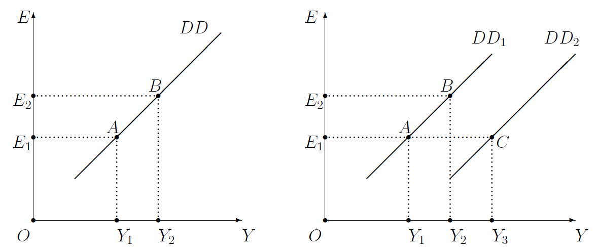
In Chapter 11, which was about the short-run and fixed exchange rates, $T$, $I$, $G$, and $q\equiv E\cdot P^*/P$ were all exogenous. In this chapter, on the other hand, $E$ is endogenous. We will, therefore, have to develop a theory that explains what makes $E$ high in certain situations and low in other situations. Nevertheless, the graphical apparatus of Chapter 11 that I have just reviewed does tell us something useful in the analysis of flexible exchange rates. It tells us that, for given (that is, pre-specified) values of the exogenous variables $T$, $I$, $G$, $P^*$, and $P$, if the goods market is in equilibrium when the endogenous variables $Y$ and $E$ are, respectively, equal to $Y_1$ and $E_1$—point $A$ in Figure 12.1 —then the goods market will also be in equilibrium at another pair of values $Y=Y_2>Y_1$ and $E=E_2>E_1$—point $B$ in figure Figure 12.1.

12.1.1 The DD Curve: slope

In other words, if there is an equilibrium outcome such that $E=E_1$ and $Y=Y_1$, as in point $A$ in Figure 12.1, there is no reason to think that it is the only equilibrium outcome. Assuming $T$, $I$, $G$, $P^*$, and $P$ are fixed, there will exist another equilibrium such that $E=E_2$ and $Y=Y_2$ as in point $B$. The collection of all such ($Y$, $E$) pairs that keep the goods market in equilibrium is the $DD$ curve. As there is a direct relation between the values of $E$ and $Y$ that keep the goods market in equilibrium when $T$, $I$, $G$, $P^*$, and $P$ are fixed, the $DD$ curve is upward-rising, as in Figure 12.1.²

Figure 12.1: If the exogenous variables $T$, $I$, $G$, $P^*$, and $P$ stay unchanged, for the goods market to be in equilibrium, any increase in $E$ must be accompanied by an increase in $Y$. This direct relation between the exchange rate and output is called the $DD$ curve. The $DD$ curve will shift to the right if $T\downarrow$, $I\uparrow$, $G\uparrow$, $P^*\uparrow$, and $P\downarrow$.

12.1.2 The DD Curve: shifts

It also follows from the last paragraph of the Section 12.1 that if $E$ remains unchanged at, say, $E_1$ in Figure 12.1, and if one or more of only these changes occur—$T\downarrow$, $I\uparrow$, $G\uparrow$, $P^*\uparrow$, and $P\downarrow$—then output would increase ($Y\uparrow$). In other words, assuming the economy was initially at the equilibrium outcome represented by point $A$ in Figure 12.1, the new equilibrium would be at a point such as $C$, with $E$ unchanged and $Y$ higher. And, as the $DD$ curve represents all possible equilibrium outcomes, if the equilibrium is no longer at point $A$, the $DD$ curve can no longer be $DD_1$. As the equilibrium has moved from $A$ to $C$, the $DD$ curve must also have moved from $DD_1$ to $DD_2$. In other words, we have established that the $DD$ curve will shift to the right if one or more of only the folowing changes occur—$T\downarrow$, $I\uparrow$, $G\uparrow$, $P^*\uparrow$, and $P\downarrow$.

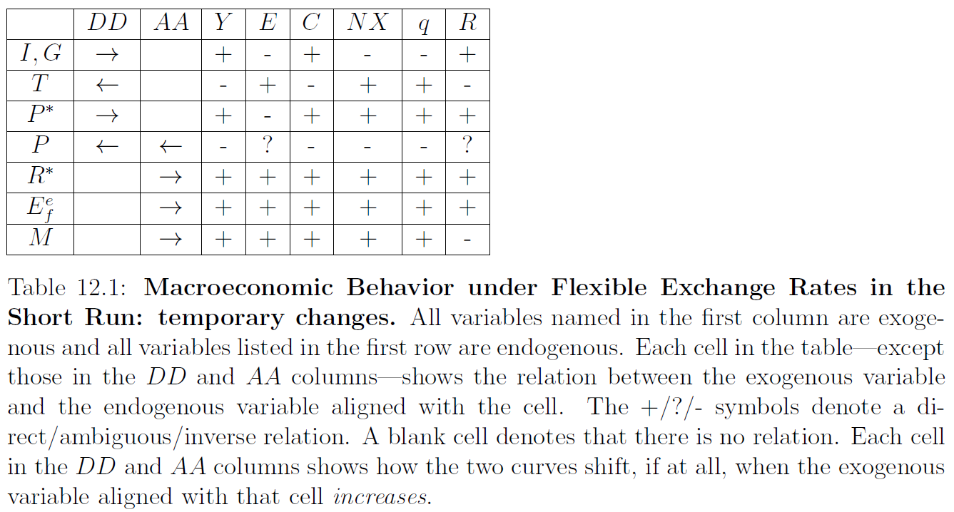
This ends my discussion of the goods market, for the time being. The $DD$-column of Table 12.1 gives a hyper-concise summary.

12.2 Asset Markets

Recall from Section 5.9.2 that equilibrium in the foreign exchange market is represented by the uncovered interest parity equation, Equation 5.13, which is \[ \fbox{$\displaystyle R=R^*+\frac{E^e_f}{E}-1.$} \tag{12.2}\]

It follows in a straightforward manner that the interest rate ($R$) will remain unchanged if $R^*$, $E_f^e$, and $E$ are unchanged. And, $R$ will increase if one or more of only the following changes occur: $R^*\uparrow$, $E_f^e\uparrow$, and $E\downarrow$.

Also, recall from Section 5.8.5 that the money market is in equilibrium when money supply ($M$) is equal to money demand ($L(R)\cdot P\cdot Y$): \[ \fbox{$M=L(R)\cdot P\cdot Y.$} \tag{12.3}\]

The two equations above can be merged into the following equation representing simultaneous equilibrium in both the money and foreign exchange markets: \[ M=L\left(R^*+\frac{E^e_f}{E}-1\right)\cdot P\cdot Y. \tag{12.4}\]

Figure 12.2: For the asset markets to be in equilibrium, if the exogenous variables $M$, $R^*$, $E_f^e$, and $P$ stay unchanged, any increase in $E$ must be accompanied by a decrease in $Y$. This inverse relation between the exchange rate and output is called the $AA$ curve. The $AA$ curve will shift to the right if $M\uparrow$, $P\downarrow$, $R^*\uparrow$, or $E_f^e\uparrow$.

12.2.1 The AA Curve: slope

The equation above has two endogenous variables ($E$ and $Y$) and four exogenous variables ($M$, $R^*$, $E_f^e$, and $P$). Suppose the magnitudes of the exogenous variables are known. Further, suppose the asset markets are in equilibrium—that is, Equation 12.4 is satisfied—for the values $E=E_1$ and $Y=Y_1$. Would this pair of values for $E$ and $Y$ be the only such pair at which Equation 12.4 is satisfied? Certainly not: there are many others.

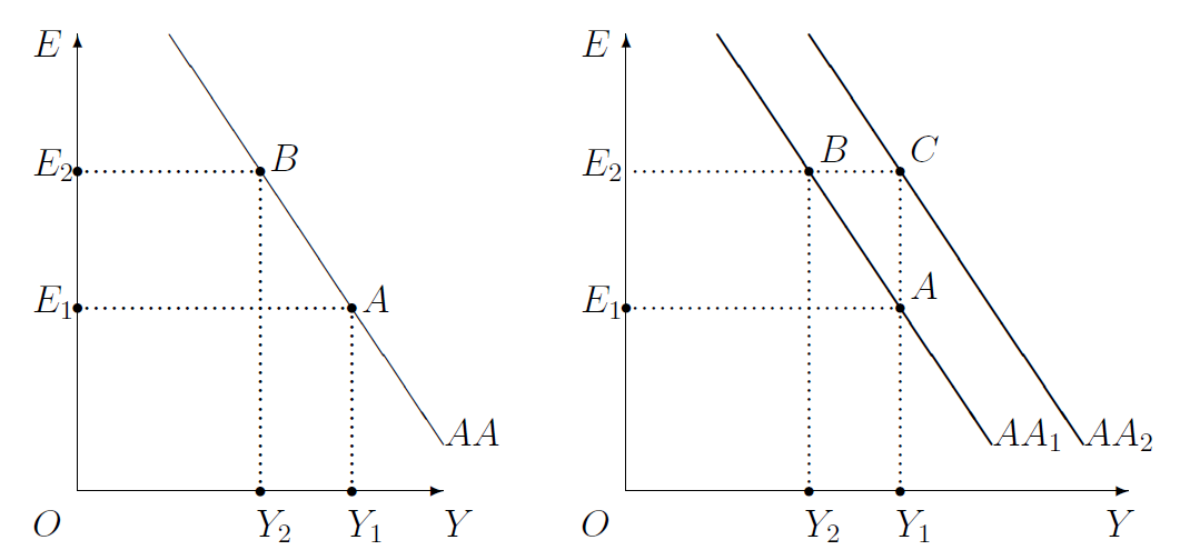
If $R^*$ and $E_f^e$ stay unchanged and the value of the foreign currency increases ($E\uparrow$), Equation 12.2 implies that the interest rate must decrease ($R\downarrow$). And, we know from Section 5.8.4.2, that this must increase people’s desire for liquidity ($L(R)\uparrow$): when the interest rate decreases people get rid of some of their interest-paying assets (such as bonds) and hold on to non-interest-paying cash instead. Now, note that Equation 12.3 implies $Y=M/(L(R)\cdot P)$. As both $M$ and $P$ are unchanged and $L(R)$ has increased, $Y$ must decrease if the asset markets are to remain in equilibrium. Therefore, we see that, if the exogenous variables ($M$, $R^*$, $E_f^e$, and $P$) are unchanged, and if the asset markets are in equilibrium when $E=E_1$ and $Y=Y_1$, then the asset markets will also be in equilibrium for some higher value of $E$—such as $E=E_2$ in Figure 12.2 —and some lower value of $Y$—such as $Y=Y_2$ in Figure 12.2.

That is, if initially the asset markets are in equilibrium and $E=E_1$ and $Y=Y_1$ as in point $A$ in Figure 12.2, this will not be the only asset markets equilibrium outcome. Assuming $M$, $R^*$, $E_f^e$, and $P$ are fixed, there will exist other equilibrium in which $E=E_2$ and $Y=Y_2$ as in point $B$. The collection of all such outcomes that keep the asset markets in equilibrium is the $AA$ curve. As there is an inverse relation between the values of $E$ and $Y$ that keep the asset markets in equilibrium when $M$, $R^*$, $E_f^e$, and $P$ are fixed, the $AA$ curve is downward-sloping, as in Figure 12.2.³

Figure 12.3: The short-run equilibrium under flexible exchange rates is at $Q$, the intersection of the $DD$ and $AA$ curves.

12.2.2 The AA Curve: shifts

Let us return to point $B$ in Figure 12.2, where the asset markets are in equilibrium. Let us consider what would happen if the money supply increases ($M\uparrow$), the other exogenous variables ($R^*$, $E_f^e$, and $P$) remain unchanged. Is it possible that at the new equilibrium the exchange rate is still at $E=E_2$? We know from Equation 12.2 that the interest rate ($R$) will not change. Therefore, $L(R)$ will not change. Therefore, as Equation 12.3 implies $Y=M/(L(R)\cdot P)$, the increase in money supply will lead to an increase in output ($Y\uparrow$). That is, when $M$ increases, there indeed would exist a new equilibrium such that $E=E_2$, as before, but with an output that’s higher than before. In other words, the increase in $M$ pushes the outcome from $B$ to $C$.

Following the same line of reasoning, it can be shown that if domestic prices fall ($P\downarrow$), the other exogenous variables ($R^*$, $E_f^e$, and $M$) remain unchanged, and the exchange rate stays unchanged at $E=E_2$, then neither $R$ nor $L(R)$ will change, and, consequently, output will increase ($Y\uparrow$).

Next, what would happen if the foreign interest rate increases ($R^*\uparrow$), the other exogenous variables ($M$, $E_f^e$, and $P$) remain unchanged, and the exchange rate also stays unchanged at $E=E_2$. We know from Equation 12.2 that the interest rate must increase ($R\uparrow$). Therefore, as we saw in the opening paragraph of this section, the people’s desire for liquidity must decrease ($L(R)\downarrow$). Therefore, as $Y=M/(L(R)\cdot P)$, it follows that output must increase ($Y\uparrow$).

The previous paragraph could be repeated word-for-word, but with $R^*$ and $E_f^e$ changing places, to establish that an increase in the current expectation of the future value of the foreign currency ($E_f^e\uparrow$) must also lead to an increase in output ($Y\uparrow$), assuming $M$, $R^*$, $P$, and $E$ are unchanged.

In short, if $E$ stays unchanged, then, for the asset markets to remain in equilibrium, $Y$ must increase if some subset of the following ceteris paribus changes occurs: $M\uparrow$, $P\downarrow$, $R^*\uparrow$, and $E_f^e\uparrow$. In other words, assuming the economy is initially at an equilibrium outcome represented by point $B$ in Figure 12.2, the new equilibrium would be at a point such as $C$. And, as the $AA$ curve represents all possible asset markets equilibrium outcomes, if the equilibrium is no longer at point $B$, the $AA$ curve can no longer be $AA_1$. As the equilibrium has moved from $B$ to $C$, the $AA$ curve must also have moved from $AA_1$ to $AA_2$. In other words, we have established that the $AA$ curve will shift to the right if one or more of only the following changes occur—$M\uparrow$, $P\downarrow$, $R^*\uparrow$, and $E_f^e\uparrow$. These effects are summarized in the $AA$-column of Table 12.1.

12.3 Short-Run Equilibrium

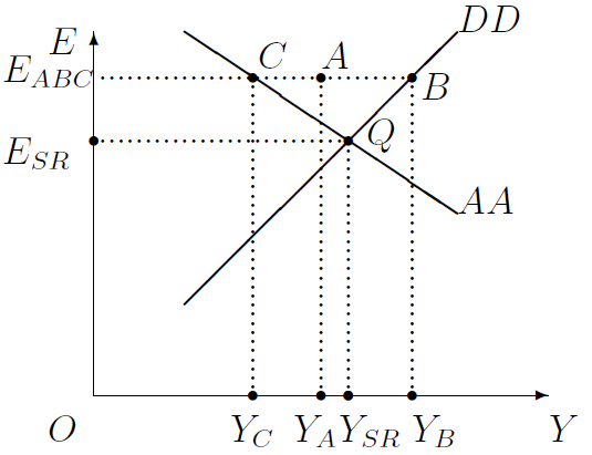
A crucial feature of the analysis presented here is the assumption that all three markets—goods, money, and foreign exchange—must be in equilibrium simultaneously. Therefore, point $A$ in Figure 12.3 cannot represent equilbrium because none of our three markets are in equilibrium when $E=E_{ABC}$ and $Y=Y_A$. Point $A$ lies neither on the $DD$ curve, which includes all outcomes that represent equilibrium in the goods market, nor on the $AA$ curve, which includes all outcomes that represent equilibrium in the asset markets, meaning the money and foreign exchange markets.

Similarly, neither $B$ nor $C$ in Figure 12.3 can be the short-run equilibrium. At $B$, which is on the $DD$ curve but not on the $AA$ curve, the goods market is in equilibrium, but not the asset markets. At $C$, the asset markets are in equilibrium but the goods market is not.

It is only at $Q$—that is, where the $DD$ and $AA$ curves intersect—that all three markets are in equilibrium. In other words, only when the exchange rate is $E=E_{SR}$ and real GDP is $Y=Y_{SR}$ does short-run equilibrium prevail. Figure 12.3 therefore shows that, if an economy’s $DD$ and $AA$ curves are known, their intersection determines the short-run equilibrium levels of the exchange rate and real income.

Figure 12.4: Short-run equilibrium under flexible exchange rates. In panel (a), $Y\uparrow$ and $E\downarrow$. In panel (d), $Y\uparrow$ and $E\uparrow$. Panels (b) and (c) show why the effect of an increase in the domestic price level ($P\uparrow$), which shifts both the $DD$ and $AA$ curves to the left, has a negative effect on output and an ambiguous effect on the exchange rate. In panel (b), $DD$ shifts a lot more than $AA$ and, as a result, $E\uparrow$. In panel (c), $DD$ shifts a lot less than $AA$ and, as a result, $E\downarrow$.

12.4 Predictions

We are now close to working out the full short-run consequences of temporary changes in our exogenous variables. We can now apply (a) our understanding that the intersection of the $DD$ and $AA$ curves determines the equilibrium values of $Y$ and $E$, and (b) our knowledge of how changes in certain exogenous variables can shift the $DD$ and $AA$ curves, to make predictions about the effects of those exogenous changes on all our endogenous variables, including $Y$ and $E$.

12.4.1 Fiscal Policy

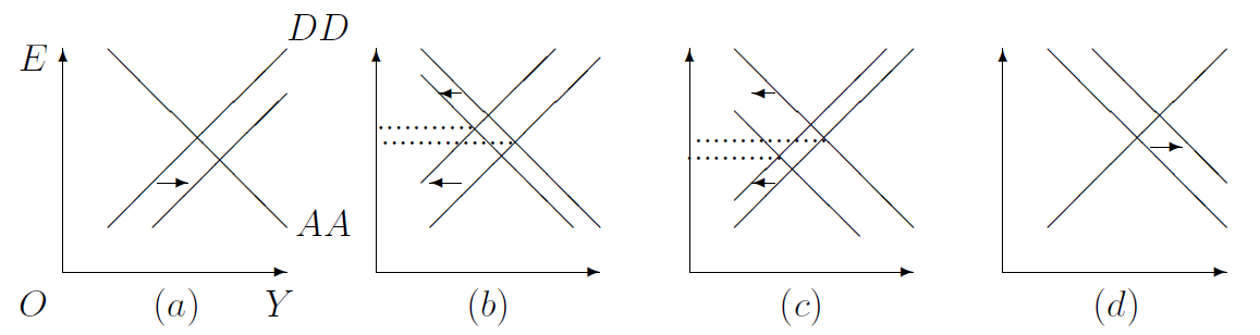
Let us begin by analysing the effects of expansionary fiscal policy, which refers to either an increase in government spending ($G\uparrow$) or a cut in taxes ($T\downarrow$) or both. We know from Section 12.1.2 and Section 12.2.2 that, as a result of these changes in fiscal policy, the $DD$ curve will shift to the right and the $AA$ curve will be unaffected. Therefore, the effects of expansionary fiscal policy can be shown by panel (a) of Figure 12.4. It follows that, real income will rise ($Y\uparrow$) and the domestic currency will appreciate ($E\downarrow$).

Therefore, disposable income must increase ($Y-T\uparrow$). And, therefore, consumption spending must increase ($C=C(Y-T)\uparrow$).

Expansionary fiscal policy cannot affect the domestic and foreign price levels ($P$ and $P^*$), which are exogenous. Therefore, the decrease in $E$ implies a decrease in the real exchange rate ($q\equiv E\cdot P^*/P\downarrow$). The decrease in the real exchange rate, which implies that foreign goods have become relatively cheaper, and the increase in disposable income, which leads to more imports, must both lead to a decrease in net exports ($NX=NX(q, Y-T)\downarrow$).⁴

Finally, note that expansionary fiscal policy cannot affect $R^*$ and $E_f^e$, which are exogenous. This, plus the decrease in $E$, together imply, as we saw in Section 12.2, that the domestic interest rate must increase ($R\uparrow$).

The reader can verify that the effects of an increase in business investment ($I\uparrow$) are identical to the effects of an increase in government spending.

To summarize, if only some subset of these exogenous changes—$I\uparrow$, $G\uparrow$, $T\downarrow$—occur, then $Y\uparrow$, $E\downarrow$, $C\uparrow$, $NX\downarrow$, $q\downarrow$, and $R\uparrow$, as shown in the rows for $I$, $G$, and $T$ in Table 12.1.

Note that these results provide an intellectual basis for the use of expansionary fiscal policy during a recession. Cutting government spending and raising taxes may represent a rare and admirable sense of responsibility and restraint in a government, but such otherwise praiseworthy behavior may not be a good idea when an economy is facing short-run trouble.

12.4.2 Foreign Price Level

The effects of an increase in foreign prices ($P^*\uparrow$) are also shown by panel (a) of Figure 12.4. Specifically, we know from Section 12.1.2} and Section 12.2.2 or from the $DD$ and $AA$ columns of Table 12.1 that the $DD$ curve shifts right and the $AA$ curve is unaffected. Therefore, $Y\uparrow$ and $E\downarrow$, as they did under expansionary fiscal policy. As taxes, which are exogenous, are unaffected, $Y-T\uparrow$, which further implies $C=C(Y-T)\uparrow$.

We know from Section 5.3 that when disposable income increases, consumption increases, but by a smaller amount. Therefore, $Y-T-C$ must increase, which implies that $Y-C$ must increase when $P^*$ increases, as the exogenous $T$ is unaffected. Now recall that the goods market’s equilibrium condition, $Y=C+I+G+NX$, implies $NX=Y-C-I-G$. As the rise in the foreign price level (a) cannot affect $I$ and $G$, which are exogenous, and (b) leads to an increase in $Y-C$, we can conclude that net exports must increase ($NX\uparrow$).

We have just seen that when $P^*$ increases, $NX$ and $Y-T$ both increase. Now recall from Section 5.6.3 that net exports ($NX=NX(q, Y-T)$) are directly related to $q$ and inversely related to $Y-T$. Given that $Y-T$ has increased, how could $NX$ have increased? The only possible explanation is that the real exchange rate must have increased, and to such an extent that $NX$ increased in spite of the increase in $Y-T$.

Finally, note that higher foreign prices cannot affect $R^*$ and $E_f^e$, which are exogenous. This, plus the decrease in $E$, together imply, as we saw in Section 12.2, that the domestic interest rate must increase ($R\uparrow$).

To summarize, if there is a ceteris paribus increase in $P^*$, then $E\downarrow$, $Y\uparrow$, $C\uparrow$, $NX\uparrow$, $q\uparrow$, and $R\uparrow$. These ceteris paribus effects are shown in the $P^*$-row of Table 12.1.

12.4.3 The Interest Rate

Now let us consider increases in $R^*$ or $E_f^e$ or both. From Section 12.1.2 and Section 12.2.2 or from the $DD$- and $AA$-columns of Table 12.1, one can check that the $DD$ curve will be unaffected and the $AA$ curve will shift to the right. These shifts are shown in panel (d) of Figure 12.4, which makes clear that real output and the exchange rate will both increase ($Y\uparrow$ and $E\uparrow$). The increase in $E$ and the fact that the exogenous prices, $P$ and $P^*$, are unaffected by changes in $R^*$ and/or $E_f^e$, together imply that the real exchange rate must have increased ($q\equiv E\cdot P^*/P\uparrow$). And, the increase in output must lead to an increase in consumption ($C=C(Y-T)\uparrow$), as taxes, which are exogenous, are unaffected by $R^*$ or $E_f^e$.

Moreover, as we saw a few paragraphs ago, $Y-C$ increases when $Y$ increases and $T$ is unchanged. Therefore, net exports, which we saw a few paragraphs back are given by $NX=Y-C-I-G$, must increase.

Now recall the money market’s equilibrium condition is given by Equation 12.3 above or $M=L(R)\cdot P\cdot Y$. This implies $L(R)=M/(P\cdot Y)$. As $M$ and $P$, which are exogenous, are unchanged, and $Y$ has increased, it follows that $L(R)$ has decreased. But we know from Section 5.8.4.2 that $L(R)$ is inversely related to $R$: when interest rates are high, people do not want to hang on to liquid cash; they’d rather buy interest-paying bonds. Therefore, the decrease in $L(R)$ implies that $R$ has increased.

To summarize, if there is a ceteris paribus increase in $R^*$ or in $E_f^e$, then $E\uparrow$, $Y\uparrow$, $C\uparrow$, $NX\uparrow$, $q\uparrow$, and $R\uparrow$. These ceteris paribus effects are shown in the $R^*$- and $E_f^e$-rows of Table 12.1 as a long row of plus ($+$) signs.

12.4.4 Monetary Stimulus

Recall that a nation’s central bank can run the printing presses at any time, and use the newly printed cash to buy financial assets such as government bonds from John or Jane Q. Public, as a result of which there would be a quick increase in $M$. What would be the short run effects of a temporary increase in the quantity of money in circulation?

The first two paragraphs of the previous section will work just fine if all mentions of $R^*$ or $E_f^e$ are replaced by $M$. Therefore, it is easy to check that $Y$, $C$, $NX$, $q$, and $E$ will all increase as a result of an increase in the quantity of money.

The only difference is that increases in $R^*$ or $E_f^e$ lead to higher domestic interest rates whereas an increase in $M$ leads to lower domestic interest rates ($R\downarrow$). To see why, recall from Equation 12.2 that $R=R^*+(E^e_f/E)-1$. An increase in $M$ depreciates the domestic currency ($E\uparrow$) and has no effect on other exogenous variables such as $R^*$ and $E_f^e$. Therefore, it follows that the domestic interest rate decreases.

To summarize, if a nation’s money supply increases—and all other exogenous variables remain unchanged—then $Y$, $C$, $NX$, $q$, and $E$ will all increase, and $R$ will decrease. This is shown in the $M$-row of Table 12.1.

The direct effect of $M$ on $Y$ is a hugely important result that is the intellectual basis of the argument in favor of expansionary monetary policy in a recession. Indeed, it is now standard practice for central banks to boost the money supply whenever a recession hits.

12.4.5 The Domestic Price Level

Finally, we need to work out how our endogenous variables respond to an increase in the domestic price level. (I have saved the toughest nut for the last!)

A quick glance at Section 12.1.2 and Section 12.2.2 or at the $DD$ and $AA$ columns of Table 12.1 shows that both the $DD$ and $AA$ curves must shift leftward when $P$ increases. These shifts are portrayed by panels (b) and (c) in Figure 12.4. It is clear that output decreases ($Y\downarrow$).

But the effect on the exchange rate is ambiguous: $E$ increases in panel (b), in which $DD$ shifts more than $AA$, but decreases in panel (c) in which $DD$ shifts less than $AA$. In other words, although an increase in the domestic price level affects the equilibrium outcome in all three markets, if the effect on the goods market is very strong compared to the effects on the money and foreign currency markets, then the value of the foreign currency increases. On the other hand, if the effect on the asset markets is stronger, then the exchange rate decreases.

Also, recall from Equation 12.2 that $R=R^*+(E^e_f/E)-1$. As an increase in $P$ cannot affect other exogenous variables such as $R^*$ and $E_f^e$, and as the effect on $E$ is ambiguous, the effect on the domestic interest rate must be ambiguous as well.

We have seen several times already that any change in $Y$ leads to similar changes in $C$ and $Y-C$, provided taxes are unaffected. Therefore, as an increase in $P$ cannot affect other exogenous variables such as $T$, the decrease in $Y$ that we saw two paragraphs back must lead to decreases in $C$ and $Y-C$. We have also seen on several occasions above that the goods market’s equilibrium condition $Y=C+I+G+NX$ implies $NX=Y-C-I-G$. Therefore, the decrease in $Y-C$ implies a decrease in net exports as well, given that $I$ and $G$, which are exogenous, are unaffected.

Note that when $P$ increases, $NX$ and $Y-T$ both decrease. Now recall from Section 5.6.3 that net exports ($NX=NX(q, Y-T)$) are directly related to $q$ and inversely related to $Y-T$. Given that $Y-T$ has decreased, how on earth could $NX$ have decreased also? The only possible explanation is that the real exchange rate must have decreased, and decreased to such an extent that $NX$ decreased in spite of the decrease in $Y-T$.⁵

To summarize, if the domestic price level increases and all other exogenous variables stay unchanged, then $Y$, $C$, $NX$, and $q$ must all decrease. The effects on $E$ and $R$ are ambiguous.

This completes my analysis of the short-run effects of temporary changes in exogenous variables in an economy that has flexible exchange rates. The results are summarized in Table 12.1.

Table 12.1: **Macroeconomic Behavior under Flexible Exchange Rates in the Short Run: temporary changes.** All variables named in the first column are exogenous and all variables listed in the first row are endogenous. Each cell in the table—except those in the $DD$ and $AA$ columns—shows the relation between the exogenous variable and the endogenous variable aligned with the cell. The +/?/- symbols denote a direct/ambiguous/inverse relation. A blank cell denotes that there is no relation. Each cell in the $DD$ and $AA$ columns shows how the two curves shift, if at all, when the exogenous variable aligned with that cell *increases*.

12.5 Conclusion

A country’s net exports (or “trade balance”) is often a controversial issue. We have seen in other contexts before that contractionary fiscal policy ($G\downarrow$ and/or $T\uparrow$) consistently leads to higher net exports. It is, therefore, a relief to see the same result in this chapter.

Although casual commentators often suggest an increase in tariffs on imported goods as a way to increase net exports, we have seen in Chapter 9} that tariffs do not affect net exports in the long run. An increase in tariffs does raise net exports in the short run under fixed exchange rates, as we saw in the last chapter. This chapter’s analysis shows the same effect is true under flexible exchange rates as well.

For more on shocks and policy variables, see Section 6.1.1.↩︎
Recall from Theorem 6.1 that if the number of endogenous variables exceeds the number of equations, the equations have many solutions. Here, we are dealing with one equation—the goods market equilibrium equation, Equation 12.1 —that has two endogenous variables, $Y$ and $E$. Therefore, it should not be a surprise that there are many pairs of values for $Y$ and $E$—such as points $A$ and $B$ and, indeed, all the other points on the $DD$ curve in Figure 12.1 —that all represent equilibrium in the goods market.↩︎
Recall from Theorem 6.1 that if the number of endogenous variables exceeds the number of equations, the equations have many solutions. Here, we are dealing with one equation—Equation 12.4 —that has two endogenous variables, $Y$ and $E$. Therefore, it should not be a surprise that there are many pairs of values for $Y$ and $E$—such as points $A$ and $B$ and, indeed, all the other points on the $AA$ curve in Figure 12.2 —that all represent equilibrium in the asset markets.↩︎
See Section 5.6.3 for more on the factors that drive a country’s net exports.↩︎
Alert readers will notice that I have used this line of reasoning before to deduce the behavior of the real exchange rate whenever disposable income and net exports move in the same direction. Disposable income is supposed to have an inverse effect on net exports. Therefore, when these two variables move together, it must be the doing of the real exchange rate. And, as the real exchange rate is the relative price of foreign goods, it has a direct effect on net exports. Therefore, if the real exchange is reversing the effect of disposable income on net exports, it must have changed in the same direction as disposable income. For instance, if $Y-T$ and $NX$ both decrease, then $q$ must also have decreased.↩︎